Modeling Patterns of Activities using Activity Curves Prafulla N. Dawadi, Diane J. Cook School of Electrical Engineering and Computer Science Washington State University, Pullman, WA
Maureen Schmitter-Edgecombe Department of Psychology Washington State University, Pullman, WA
Abstract Pervasive computing offers an unprecedented opportunity to unobtrusively monitor behavior and use the large amount of collected data to perform analysis of activity-based behavioral patterns. In this paper, we introduce the notion of an activity curve, which represents an abstraction of an individual’s normal daily routine based on automatically-recognized activities. We propose methods to detect changes in behavioral routines by comparing activity curves and use these changes to analyze the possibility of changes in cognitive or physical health. We demonstrate our model and evaluate our change detection approach using a longitudinal smart home sensor dataset collected from 18 smart homes with older adult residents. Finally, we demonstrate how big data-based pervasive analytics such as activity curve-based change detection can be used to perform functional health assessment. Our evaluation indicates that correlations do exist between behavior and health changes and that these changes can be automatically detected using smart homes, machine learning, and big data-based pervasive analytics. Keywords: Activity Curve, Smart Environments, Functional Assessment, Permuation
1
1. Introduction
2
Many pervasive computing applications such as home automation, activity aware interventions, and
3
health assessment require analyzing and understanding activity-based behavioral patterns. The performance
4
of such applications depends on the ability to correctly learn a model of general daily activity behavior from
5
a large amount of data and be able to predict when such daily behavior is likely to continue or change. These
6
big data-based approaches to activity modeling can then in turn be used to provide effective activity-aware
7
services such as improved healthcare. Email addresses: pdawadi,
[email protected] (Prafulla N. Dawadi, Diane J. Cook),
[email protected] (Maureen Schmitter-Edgecombe)
Preprint submitted to Pervasive and Mobile Computing
June 18, 2015
8
Activity recognition lies at the heart of any pervasive computing approach to modeling behavioral rou-
9
tines. An activity recognition algorithm maps a sensor reading or sequence of readings to a corresponding
10
activity label. In order to answer general questions related to daily activity patterns, such information needs
11
to be transformed to a higher-level representation. For example, questions such as how average daily activ-
12
ity patterns have changed over a year, or generally what hours did a particular individual sleep last month
13
are difficult to answer using raw output from activity recognition algorithms. However, many pervasive
14
computing applications such as home automation and health assessment require answering such questions.
15
Obtaining higher-level representations or models of activities has several additional advantages. Higher-
16
level representations can abstract variations in day-to-day activity routines. For example, wake-up times
17
in the morning may be slightly different each day even if the overall routine is fairly stable. Additionally,
18
such representations simplify the task of modeling an individual’s daily routine and at the same time make
19
visualization and interpretation of daily activity routines easy. Collecting big data sets over long periods of
20
time allows us to abstract activity models over such daily variations. As we will demonstrate in this paper,
21
such representations aid with the process of identifying long-term changes in a behavioral routine.
22
23
24
25
26
27
For example, consider the following description highlighting aspects of an individual’s routine at two different points in time: • Month of March 2012 : Sleep at 10:00 PM, get up at 6:00 AM, eat breakfast at 7:00 AM, eat lunch at 12:00 PM, go out for a walk at 4:00 PM, and dine at 8:00 PM. • Month of September 2013 : Sleep at 8:00 PM, wake up frequently during the night, get up at 10:00 AM, no breakfast, eat lunch at 11 AM, no going out for a walk, and dine at 7:00 PM.
28
Note that each of these sample activity-based descriptions is aggregated over a one-month period and
29
therefore describes a general routine that is maintained over a prolonged period of time. Based on these
30
descriptions we also note changes in the routine from the first observation to the second. From this example,
31
we can infer that by September 2013 the observed individual was experiencing disturbances in sleep, was
32
skipping meals, and stopped exercising. Determining if the overall daily activity patterns has changed may be
33
difficult based only on the raw sensor data or even based on event-by-event labels from an activity recognition
34
algorithm. Such questions can be more easily answered by comparing two higher-level representations of
35
these activity patterns.
36
In our current work, we propose a novel activity curve to model an individual’s generalized daily activity
37
routines. The activity curve modeling algorithm uses activity-labeled sensor events to learn a higher-level
38
representation of the individual’s regular routine. These activity labels are automatically-recognized using an
39
activity recognition algorithm. We also introduce a Permutation-based Change detection in Activity Routine
40
(PCAR) algorithm to compare activity curves between different time points in order to detect changes in an
41
activity routine. To validate our algorithm, we make use of longitudinal smart home sensor data collected 2
42
by monitoring everyday behavior of residents over two years. Finally, we demonstrate how the activity curve
43
and the PCAR algorithm can be used to perform important pervasive computing tasks such as automated
44
assessment of an individual’s functional health.
45
2. Related work
46
The work that we describe in this paper is unique in its ability to automatically characterize behavioral
47
routines based on recognized activities and to detect changes in generalized routines over time. However,
48
other work has focused on alternative approaches to recognizing and discovering daily activity routines and
49
two-sample tests to detect changes between two sample populations similar to the core component of the
50
proposed PCAR algorithm. Additionally, other studies have investigated the relationship between changes
51
in activity patterns and changes in health using the statistical and visualization techniques.
52
Discovering activity routines: Researchers have studied the problem of automated discovery and recog-
53
nition of daily activity routines using the data collected from wearable sensors [1, 2], GPS signals [3] and
54
mobile phones [4] using algorithms such as topic modeling [1] and collaborative filtering [5]. In these ap-
55
proaches, raw sensor data are converted to a bag-of-words representation which contains the histogram of
56
activity label occurrences or histogram of location/proximity information. Data from wearable sensors can
57
be used to discover daily routines such as having lunch and brushing teeth [1]. Similarly, data from mobiles
58
phones can be used to recognize routines such as commuting to office and working.
59
In contrast to these earlier works that focus on discovering and recognizing daily activity routines from
60
sensor data, our focus is to model the discovered and recognized daily activity routines using an activity
61
curve model. The proposed activity curve model is a generic model that can be calculated both from the
62
output of an activity recognition algorithm as well as using the algorithms mentioned in the aforementioned
63
studies. Furthermore, our proposed model facilitates answering more complex questions related to activity
64
routines such as whether changes in an activity routine have occurred or not. In our current work, the
65
proposed activity curve model uses the output from an activity recognition algorithm.
66
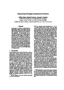
Visualization of activity routines: Researchers have proposed visualization techniques to visualize daily
67
activity patterns. For example, Galambos et al. [6, 7] developed methods to visualize activity level, time
68
spent away from home, deviations in activities of daily living, and behavioral patterns. Similarly, other
69
researchers have developed techniques to visualize deviations in activity routines and behavioral patterns
70
using smart home sensors [8, 9]. These methods provide a tool to understand sensor-monitoring data and to
71
study daily activity routines. However, these approaches rely on manual inspection of the data in order to
72
make any higher-level conclusions regarding daily routines.
73
Two-sample test: The two-sample test is a widely used statistical analysis tool to compare between two
74
sample populations. Classical two-sample tests such as the t-test are used to compare the means of two
3
75
populations having the same or different variances. However, the t-test is a parametric test that is limited
76
to comparing between two Gaussian distributions. Other examples of non-parametric classical versions of
77
two-sample tests are the Wald-Wolfowitz runs test, the Anderson-Darling test and the Kolmogorov-Smirnov
78
test [10].
79
Recently, Maximum Mean Discrepancy (MMD) was proposed as another non-parametric two-sample test
80
technique [11]. MMD compares the means of two distributions in a universal reproducing kernel Hilbert space
81
and has superior performance to several of the classic two-sample tests. However, the superior performance
82
of MMD relies on a valid choice of a kernel and kernel width, and recommendations have been made in
83
the literature for obtaining optimal performance with MMD [12]. Similarly, the Least Squares Sample Test
84
(LSTT) technique has been proposed in the literature to make use of permutation to perform two-sample
85
tests [13]. In the LSTT based two-sample test, divergence is estimated using the density ratio estimation
86
technique and the permutation-based technique is used to test the significance of the estimated divergence.
87
Such permutation-based tests are preferable because they are data-centric approaches that make inferences
88
directly from data.
89
The proposed PCAR algorithm detects significant changes in activity curves based on a permutation-
90
based two-sample test using symmetric Kullback-Liebler divergence as a distance metric. Our proposed
91
method to detect changes in activity routines has some similarities with activity tracking algorithms that
92
have been previously proposed [14, 15]. These proposed activity-tracking algorithm discovers and tracks
93
changes in sensor sequence patterns for the purpose of adapting home automation strategies. In contrast,
94
our method tracks changes in the distribution of automatically-recognized activity patterns.
95
Relationship between changes in activity routines and health: Researchers have developed functional
96
assessment algorithms based on different parameters of everyday abilities. These researchers have studied
97
correlations between everyday abilities and corresponding standard clinical measurements. Researchers have
98
correlated sensor measurements of sleep patterns, gait, activity rhythms, indoor activities and outings, and
99
mobility with standard clinical measurements such as MMSE and self-report data. For example, Paavilainen
100
et al. [16] compared the changes in circadian rhythm of activities of older adults living in nursing homes
101
with clinical observations of the health status of subjects. In other work, Robben et al. [17, 18, 19] studied
102
the relationship between different high-level features representing the location and transition patterns of an
103
individual’s indoor mobility behavior, namely the frequency, duration and times being carried out, with the
104
Assessment of Motor and Process Skills (AMPS) scores [20]. Other researchers have studied the relationship
105
between walking speed and the amount of in-home activity among healthy older adults and older adults with
106
Mild Cognitive Impairment (MCI). These researchers found out that coefficient of variation in the median
107
walking speed was higher in the MCI group as compared with the healthy group. However, none of these
108
works considered parameters reflecting the performance of activities of daily living.
4
Figure 1: Example activity distributions calculated at 60 minute time intervals. The figure models three possible activities: sleep, bed toilet transition, and an “other” activity. An activity curve is thus the compilation of all of these activity distributions.
109
Other researchers have developed functional assessment algorithms based on performance of an individual
110
in a fixed set of activities. They have correlated the performance in these activities with the direct observation
111
of participants completing the ADLs. In one such work, Dawadi et al.[21, 22] proposed learning algorithms
112
to obtain activity performance measures of simple and complex ADLs from sensor data and correlated
113
them with validated performance measures derived from direct observation of participants completing the
114
ADLs. They also studied the relationship between sensor-detected activity performance measures and overall
115
cognitive health. In another work, Hodges et al. [23] correlated sensor events gathered during a coffee-making
116
task with an individual’s neuropsychological score. Similarly, in an another research effort by Riboni et
117
al.[24] researchers developed a Fine-grained Abnormal BEhavior Recognition (FABER) algorithm to detect
118
abnormal behaviour using a statistical-symbolic technique. These researchers hypothesize that such abnormal
119
activity routines may indicate the onset of early symptoms of cognitive decline.
120
3. Activity curve
121
An activity curve is a model that represents an individual’s generalized activity routine. We are interested
122
in modeling activity routines for a day-long period but this time period can be changed as needed. The
123
activity curve uses automatically-recognized activity labels to express daily behavioral characteristics based
124
on the timing of recognized activities.
125
We assume that a continuous sequence of time-stamped sensor events is available. We use an activity
126
recognition algorithm to annotate each of these sensor events with an activity label. Activity recognition
127
algorithms map a sequence of sensor events {e1 , e2 , . . . , en } onto the corresponding activity label Ai , where
128
the label is drawn from the predefined set of activity classes A = {A1 , A2 , . . . , An }.
129
We note that prevalence of common activities differs by the time of day. For example, the “sleep” activity
130
dominates the prevalent distribution of activities at midnight and the “cook breakfast” and “eat breakfast”
131
activities dominate the early morning hours. To capture such differences in activity patterns throughout the
132
day, we segment the day-long observation period into m equal-size consecutive windows, or time intervals,
5
133
and define probability distributions over activities, or activity distributions, for each of these time intervals
134
(see Figure 1 for an example). An activity curve is a compilation of these activity distributions for the entire
135
day-long period.
136
We also note that our activity routines tend to vary from one day to the next. For example, we may wake
137
up at 6:30 AM and eat breakfast at 7:15 AM one day while we might wake up at 7:30 AM and eat breakfast at
138
8:00 AM the next day. In order to generalize our model over such day-to-day variations in activity routines,
139
we will define the notion of an aggregated activity curve that is calculated over an aggregation window of x
140
days.
141
Definition 1. Given a time interval t, an activity distribution models the daily routine based on the predefined
142
set of activities A as a probability distribution over activities in A. The probability distribution can be
143
estimated from sample data based on the normalized time an individual spends on a predefined set of n
144
activities during time intervals t as observed during one or more days.
145
An activity distribution for time interval t is a n-element set Dt = {dt,1 , dt,2 , . . . , dt,n } whose length is
146
equal to that of the activity set A. The ith element in an activity distribution, dt,i , represents the probability
147
of performing activity Ai during time interval t.
148
To model a person’s overall daily activity routine, we use m activity distributions corresponding to each
149
of the m time intervals. We can then construct an activity curve by collecting activity distributions that
150
model daily activity patterns at all different times of the day.
151
Definition 2. An activity curve C is the compilation of activity distributions Dt ordered by time interval t.
152
The length of an activity curve is m. We refer to the model that compiles activity distributions as an
153
“activity curve” because if we consider the activity distribution of activity Ai for all time intervals 1, 2, . . . , m,
154
these activity distributions form a curve that represents the “fraction of a time” that an individual is likely
155
to perform activity Ai over successive time intervals.
156
ˆ t for time interval t by aggregating activity distribuWe calculate an aggregated activity distribution D
157
tions Dk,t (1 ≤ k ≤ x) over an aggregation window of x days. If D1,t , D2,t , . . . , Dx,t are activity distributions
158
for the tth time interval aggregated over a window of x days and follow normal distributions, then we can
159
define an aggregated activity distribution as follows.
160
ˆ t at time interval t is the maximum likelihood estimate of Definition 3. An aggregated activity distribution D
161
the mean that is obtained from activity distributions Dk,t (1 ≤ k ≤ x) that fall within an aggregation window
162
of size x.
163
ˆ t at time interval t as show in Equation 1. We can write the aggregated activity distribution D ˆt = D
x X Dk,t k=1
6
x
(1)
Avg. time spent in activity in that interval (normalized)
1.0
BedToilet Sleep Other Activity
0.8
0.6
0.4
0.2
0.0
0
50
100
150
200
250
300
Index of a time interval Figure 2: An example aggregated activity curve that models three different activities: sleep, bed toilet transition, and an “other” activity. This sample aggregated activity curve was derived using x = three months of actual smart home data. Aggregated activity distributions were calculated at 5 minute time intervals, (m = 288). In this graph, the time interval at index 0 represents 12:00 AM.
164
Definition 4. An aggregated activity curve is the compilation of aggregated activity distributions obtained
165
over an aggregation window of size x.
166
If Σ = {C1 , C2 , C3 , . . . , Cx } is a set of activity curves over an aggregation window of size = x days, we
167
can represent an aggregated activity curve over Σ as C Σ . The aggregated activity curve C Σ compiles the
168
ˆ t . Figure 2 illustrates an example of an aggregated activity curve that aggregated activity distributions, D
169
models three different activities: sleep, bed toilet transition, and other.
170
4. Activity distribution distance
171
We calculate the distance between two activity distributions using the Kullback-Leibler (KL) divergence
172
measure. We assume that the activity distributions model the same activity set A for the same time
173
interval size and aggregation window size. The KL divergence between two activity distributions D1 =
174
{d1,1 , d1,2 , . . . , d1,i , . . . , d1,n } and D2 = {d2,1 , d2,2 , . . . , d2,i , . . . , d2,n } is defined as shown in Equation 2.
DKL (D1 ||D2 ) =
n X i=1
d1,i log
d1,i d2,i
(2)
175
We note that the standard KL distance metric is a non-symmetric measure of the differences between
176
two probability distributions D1 and D2 . Therefore, we use a symmetric version of the Kullback-Leibler
177
divergence between activity distributions D1 and D2 , which is defined as shown in Equation 3. Throughout 7
178
the remainder of the paper, our discussion of KL divergence will refer to this symmetric version of the KL
179
divergence measure. SDKL (D1 ||D2 ) = DKL (D1 ||D2 ) + DKL (D2 ||D1 )
(3)
180
Before defining the distance between two activity curves C1 and C2 of length m, we first need to align
181
the activity distributions in the activity curves (this is described in Section 6). As a result of the alignment
182
step, we obtain a vector of alignment pairs Γ = (p, q) of length l = |Γ| that aligns an activity distribution at
183
time interval p
184
of activity curve C2 .
185
186
(1 ≤ p ≤ m) of activity curve C1 with activity distribution at time interval q
(1 ≤ q ≤ m)
We calculate the total distance, SDKL (C1 ||C2 ), between two activity curves, C1 and C2 , as the sum of distances between each aligned activity distribution for the two activity curves, as shown in Equation 4.
SDKL (C1 ||C2 ) =
l X
SDKL (D1,p ||D2,q ) such that Γα = (p, q)
(4)
α=1
187
where D1,p and D2,q are the activity distributions that belong to activity curves C1 and C2 at time intervals
188
p and q, respectively.
189
5. Determining the size of an aggregation window
190
Daily activity routines are performed differently from one day to the next. As a result, the daily activity
191
curve that models these activity routines will vary from one day to the next. We want to calculate an
192
aggregated activity curve that generalizes over minor day-to-day variations while still capturing the typical
193
routine behavior. When determining the appropriate size of an aggregation window, our goal is to find the
194
smallest possible number of days that is considered stable. We determine that an aggregated activity curve
195
is stable if the shape of the curve remains mostly unchanged when more days are added to the aggregation
196
window. By keeping the aggregation window small, our model can be more sensitive to significant changes
197
in routine behavior. If the window is too small it will not be general enough to encompass normal variations
198
in daily routines. We propose Algorithm 1 to determine the minimum length of an aggregate window that
199
is required to calculate a stable, representative aggregated activity curve for a particular time interval. We
200
choose the minimum aggregate window size xmin such that no smaller window would ensure the stability
201
criterion.
202
To determine the ideal aggregation window size, we start with a window of size x = 2 and consider
203
the corresponding aggregated activity curve C Σ , aggregated from the set of individual activity curves Σ =
204
Σ {C1 , . . . , Cx }. We estimate the distance between CxΣ and Cx+1 . If the distance is greater than a predefined
205
Σ Σ Σ threshold T , we increase the window size. Therefore, if SDKL (CxΣ ||Cx+1 ) < T and SDKL (Cx+1 ||Cx+2 ) < T,
8
206
then x is selected as the representative aggregation window size, otherwise we increase size of the aggregation
207
window by one and repeat the process. This process is shown in Algorithm 1. Algorithm 1 AggregationSize(Σ, T ) 1: // Calculate the minimum size of an aggregation window. 2: Σ = {C1 , C2 , . . . , CN } for each of the N days in the input data. 3: // Return the minimum aggregation window size. 4: initialize x = 2 5: repeat: 6: Create CxΣ , aggregated activity curve for window size x. Σ , aggregated activity curve for window size x + 1. 7: Create Cx+1 Σ 8: Create Cx+2 , aggregated activity curve for window size x + 2. Σ 9: Compute d1 = distance between two aggregated activity curves SDKL (CxΣ ||Cx+1 ). Σ Σ 10: Compute d2 = distance between two aggregated activity curves SDKL (Cx+1 ||Cx+2 ). 11: if d1 > T and d2 > T , then x = x + 1 12: else return x 13: until x < N
208
6. Activity curve alignment
209
In order to compute similarity (or distance) between two activity curves, we need to compare each of the
210
activity distributions that belong to these two activity curves. However, we first need to determine which
211
pairs of distributions to compare by considering alternative distribution alignment techniques. Activity curve
212
alignment can be performed based on aligning the same time of day between two curves. Alternatively, we
213
can try to maximally align the activity occurrences between two curves before performing such a comparison.
214
Here we provide details for these two alignment techniques that we use in our work.
215
6.1. Time interval-based activity curve alignment
216
The time interval-based activity curve alignment technique presumes that distributions between two
217
curves should be aligned based on time of day and thus aligns activity distributions between two activity
218
curves if the time intervals are the same. In essence, this method does not make any extra effort to align
219
activities that occur at different times in the distribution, but simply compares the activity distributions
220
based on time of day alone.
221
If C1 and C2 are two activity curves of length m, the time interval-based activity distribution alignment
222
method aligns the corresponding activity distributions using a vector of alignment pairs, Γ = (r, r). This
223
technique aligns an activity distribution at time interval r
224
distribution at time interval r
(1 ≤ r ≤ m) of activity curve C1 with activity
(1 ≤ s ≤ m) of activity curve C2 .
9
225
6.2. Dynamic time warping-based activity curve alignment
226
A person’s routine may be relatively stable, even though there are minute changes in the time an activity
227
occurs or the duration of a particular activity. For example, an individual may sleep at 10:00 PM one day,
228
an hour earlier at 9:00 PM the next day, an hour later at 11:00 PM a few days later, and eventually go back
229
to sleeping at 10:00 PM. Aligning activity distributions using dynamic time warping allows us to maximally
230
align common activities before comparing two activity curves. Such an alignment accommodates activity
231
time changes that are shifted temporally backward (for example, an hour earlier), forward (for example,
232
an hour later), expanded (longer duration), compressed (shorter duration), or not changed at all from one
233
day to another. We optimize activity alignment using Dynamic Time Warping(DTW) to align distributions
234
between two activity curves.
235
Dynamic time warping finds an optimal alignment or warping path between activity curves. This optimal
236
warping path has minimal total cost among all possible warping paths. We use the symmetric KL distance
237
metric that we previously mentioned to compute this warping path. The warping path has the following
238
three main properties:
239
240
• Boundary property: The first and last elements (activity distributions) from the two activity curves are always aligned with each other.
241
• Monotonicity property: Paths are not allowed to move backwards.
242
• Step size property: No activity distributions are omitted from the curve alignment.
243
We also note that due to the monotonicity property, DTW does not allow backward alignments. However,
244
as we have seen in practice, activity distributions can be shifted temporally backward and/or temporally
245
forward. Therefore, we modify the standard approach to perform two independent iterations of DTW:
246
• In forward dynamic time warping, we start from the first activity distribution and move forward in
247
time toward the last activity distribution to find an optimal alignment between activity curves that
248
are similar in the forward time direction.
249
• In backward dynamic time warping, we start from the last activity distribution and move backward in
250
time toward the first activity distribution to find an optimal alignment between activity curves that
251
are similar in the backward time direction.
252
If C1 and C2 are two activity curves of length m, the DTW-based activity distribution alignment outputs
253
two alignment vectors, Γf orward = (u, v) of length lf orward , and Γbackward = (r, s) of length lbackward ,
254
respectively. The forward DTW aligns an activity distribution from curve C1 at time interval u (1 ≤ u ≤ m)
255
with an activity distribution from curve C2 at time interval v
256
aligns an activity distribution from curve C1 at time interval r 10
(1 ≤ v ≤ m). Similarly, the backward DTW (1 ≤ r ≤ m) with an activity distribution
257
from curve C2 at time interval s (1 ≤ s ≤ m). The DTW method outputs whichever vector, Γf orward
258
or Γbackward , that results in the maximal alignment between the two distributions and thus minimize the
259
difference. We will utilize these two different alignment techniques in our PCAR algorithm to detect changes
260
between two aggregated activity curves and calculate change scores.
261
7. PCAR
262
Based on our notion of an activity curve, we now introduce our Permutation-based Change Detection in
263
Activity Routine (PCAR) algorithm. This algorithm identifies and quantifies changes in an activity routine.
264
PCAR operates on the assumption that daily activities are scheduled according to a routine and are not
265
scheduled randomly. For example, we regularly “wake up”,“bathe” and “have breakfast” in the morning
266
and “dine” and “relax” in the evening. In contrast, we rarely dine in the middle of night. Such regularities
267
are useful, for example, to determine if there are significant changes in lifestyle behavior that might indicate
268
changes in cognitive or physical health.
269
7.1. Permutation-based two-sample test
270
PCAR identifies significant changes in an activity routine using a two-sample permutation test [25]. The
271
permutation-based technique provides a data-driven approach to calculate an empirical distribution of a
272
test statistic. The empirical distribution of a test statistic is obtained by calculating the test statistic after
273
randomly shuffling (rearranging) the data a specified number of times. The permutation-based test is exact
274
if the joint distributions of rearranged samples are the same as the joint distribution of the original samples.
275
In other words, the samples are exchangeable when the null hypothesis is true. This type of test allows us
276
to determine the significant difference between two aggregated activity curves.
277
We use a permutation-based test to perform a two-sample homogeneity test. In a two-sample homogeneity
278
test, we test the null hypothesis that the two samples come from the same probability distribution versus
279
the alternate hypothesis that they come from different probability distributions.
280
7.2. Changes in activity distributions
281
We use the permutation-based two-sample test to determine whether there is a significant change among
282
a set of activity distributions at a particular time interval. We formulate the null hypothesis that the set of
283
activity distributions comprising two activity curves are identical versus the alternative hypothesis that the
284
set of activity distributions is significantly different between the two aggregated activity curves.
285
286
287
288
ˆ 1,t and We test the hypothesis of a significant change between two aggregated activity distributions, D ˆ 2,t . D ˆ 1,t ||D ˆ 2,t ) between the two • Calculate the test statistic: Calculate the test statistic Distt = SDKL (D aggregated activity distributions. 11
Figure 3: The permutation-based steps to detect changes in the activity curve. The first step is to compute the test statistic from the original samples. In the second step, the samples are rearranged N times and the test statistic is calculated for each arrangement. In the third step, significance testing is performed by comparing the test statistic obtained from the original (unpermuted) set of data with the the test statistic obtained from the permuted data. Finally, a change score is calculated by counting the number of significant changes in activity distributions.
289
• Permutation: Randomly shuffle individual activity distributions between the two aggregated distribu-
290
ˆ 1,t and D ˆ 2,t . Calculate the KL divergence between tions and recalculate the aggregated distributions D
291
ˆ 1,t ||D ˆ 2,t ). Repeat the process a specified ˆ t = SDKL (D the new aggregated activity distributions Dist
292
ˆ t. number of times to obtain an empirical distribution of KL divergence (the test statistic), Dist
293
ˆ 1,t and D ˆ 2,t calculate the p-value • Significance testing: To test if a significant difference exists between D
294
by calculating the number of times the test statistic from the permuted sample is equal to or greater
295
ˆ t . If a small p-value is obtained, than the original test statistic Distt , in the empirical distribution Dist
296
reject the null hypothesis in favor of alternative hypothesis. This is shown in Equation 5.
pperm =
ˆ t > Distt #Dist #permutations
(5)
297
ˆ t is the empirical distribution of the test statistic at the tth time interval. We reject the null where Dist
298
hypothesis that no changes have occurred at a significance level of α = 0.01.
299
7.3. Changes in activity curves
300
We now extend the technique of detecting significant changes between activity distributions to quantify
301
the difference in activity routine observed from two separate aggregation windows, W1 and W2 , each of size
302
x days. To do this, PCAR counts the total number of significant differences between the individual activity
303
distributions within window W1 and the distributions within window W2 to output a change score that
304
quantifies the significant changes observed among the activity curves. Figure 3 demonstrates the three main
305
steps involved in detecting changes in an activity curve using the permutation-based method.
12
306
PCAR calculates a sum, S, over changes that are detected between activity curve distributions for each
307
individual time interval. In order to identify the time intervals at which changes in the activity distributions
308
comprising the aggregated activity curves are deemed significant, PCAR performs the following steps:
309
• Permutation: Calculate the empirical distributions of the test statistic (KL divergence) by permuting
310
and comparing the individual activity distributions within the two aggregation windows W1 and W2
311
at each time interval using the method summarized in Algorithm 2.
312
• Alignment: Calculate the two aggregated activity curves C1 and C2 using the activity distributions
313
aggregated for each time interval over windows W1 and W2 . Align curves C1 and C2 using one of the
314
alignment techniques described in the previous section to generate the alignment vector Γ = (u, v).
315
• Calculate the test statistic: For each alignment pair (u, v) ∈ Γ, calculate the test statistic Distu,v
316
between the aggregated activity distribution at time interval u of activity curve C1 and the aggregated
317
activity distribution at time interval v of C2 .
318
• Significance testing: To test if there is a significant change between activity distributions at time
319
intervals u and v, calculate the p-value based on the the number of times the test statistic from the
320
permuted sample is equal to or greater than the original test statistic. The steps are summarized in
321
Algorithm 3.
322
We note that we compare at least m activity distributions during this process where m is the number
323
of aggregated activity distributions in an activity curve. To control the False Discovery Rate (FDR) at
324
level α∗ (α∗ = 0.01), we apply the Benjamini-Hochberg (BH) method [26]. The BH method first orders the
325
p-values, p(1) , p(2) , . . . , p(k) , . . . , p(m) , in ascending order and for a given value of α∗ , the BH method finds
326
the largest k such that p(k) ≤ k × αm . The BH algorithm rejects the null hypothesis corresponding to p(i) if
327
i ≤ k. If a significant change is detected between aligned activity distributions, PCAR increments its change
328
score, S, by one. PCAR generates two different change scores based on the alignment techniques that are
329
employed: either the same index alignment or the DTW-based alignment.
330
8. Use of activity curves for smart functional assessment: A case study
∗
331
An activity curve model provides a big data-based tool for representing a longer-term behavioral model.
332
Such a tool is valuable for a variety of applications including human automation, health monitoring, and
333
automated health assessment. In this section, we explain how the activity curve model and the PCAR
334
algorithm can be instrumental in performing automated functional assessment.
335
Activities of daily living such as sleeping, grooming, and eating are essential everyday functions that
336
are required to maintain independence and quality of life. Decline in the ability to independently perform 13
Algorithm 2 EmpiricalDistribution(Σ1 , Σ2 , NP ) ˆ of the test statistic. 1: // Build empirical distribution Dist 2: Σ1 , Σ2 = two sets of activity curves 3: Np = number of permutations ˆ as Np × m matrix 4: initialize Dist . m is # activity distributions in the activity curves 5: initialize i = 0 6: while i < Np do : 7: Shuffle the activity curves. 8: Generate aggregated activity curves C Σ1 and C Σ2 by aggregating the distributions in Σ1 , Σ2 9: Using the time interval-based alignment technique, align the two aggregated activity curves to obtain an alignment vector Γ. 10: for all alignment pairs (u, u) in Γ do : 11: Find a distance SDKL (D1,u ||D2,u ) between uth activity distributions in two activity curves. ˆ at location [i, u]. 12: Insert SDKL (D1,u ||D2,u ) to empirical distribution Dist 13: end for 14: i = i+1 15: end while ˆ 16: return Dist
337
these ADLs has been associated with a host of negative outcomes, including placement in long-term care
338
facilities, shortened time to conversion to dementia, and poor quality of life for both the functionally impaired
339
individuals and their caregivers [27, 28, 29].
340
We use smart home sensor data to derive activity curves that model the activity routines of a smart
341
home resident. Our PCAR algorithm detects changes in those activity routines. We note that changes in
342
ADL patterns are one of the many forms of behavioural changes that are frequently associated with changes
343
in cognitive and physical health. We hypothesize that activity curve will allow us to detect changes in ADL
344
patterns which possibly can provide valuable information about a change in the health condition. To validate
345
our automated assessment technique, we utilize smart home sensor data that was collected from real world
346
smart home test beds with older adult residents. We apply robust activity recognition algorithms [30, 31] to
347
label these sensor-monitored data with the corresponding activity labels. ˆ Algorithm 3 PCAR(Σ1 , Σ2 , Dist) 1: Σ1 , Σ2 = two sets of activity curves 2: //Return a change score S 3: C1 = AggregateActivityCurves(Σ1 ) 4: C2 = AggregateActivityCurves(Σ2 ) 5: Γ = AlignCurves(C1 , C2 ) 6: for all alignment pairs (u, v) in Γ do : 7: Calculate SDKL (D1,u ||D2,v ) between activity distribution D1,u ∈ C1 and D2,v ∈ C2 . ˆ 8: Perform significance testing of estimated distance by querying Dist. 9: if change is significant : 10: S =S+1 11: end for 12: return S
14
348
8.1. Synthetic dataset
349
First, we validate the performance of the proposed PCAR algorithm by running it on a synthetic activity
350
curve. We create a synthetic activity curve by compiling synthetic activity distributions. The synthetic
351
activity distribution models the patterns of two activities, an arbitrary activity A and an “other” activity.
352
353
354
355
We generate synthetic activity distributions for each time interval t for N days by applying the following three steps. Here l represents the length of each time interval. • Generate a random value p
(0 ≤ p ≤ l), which represents the average time that is spent in performing
activity A during time interval t.
356
• Generate two vectors, S and S 0 , each of length N . Generate the vector S from a normal distribution
357
i.e. S ∼ Normal(p, 1). Each element of vector S 0 is generated by subtracting the corresponding value
358
in S from l i.e l − s ∈ S 0 .
359
• Create an activity distribution that models patterns of two activities at a time interval t. The elements
360
of the activity distribution is [s, l − s]. We combine these individual synthetic activity distributions at
361
different time intervals into activity curves. When we introduce an activity change, we multiply the
362
average time spent performing an activity A by a constant factor in each time interval.
363
Using the aforementioned method, we create two different sets of activity curves. The first set Y does
364
not contain any changes and another different set of daily activity curves Z contains changes in all activity
365
distributions every 90 days. We run the PCAR algorithm on an aggregated activity curve of size 90 days
366
using the time interval index alignment. PCAR successfully detects all changes in the dataset where activity
367
changes were made and does not produce any false positives in the synthetic dataset that does not contain
368
changes.
369
8.2. Experimental setup
370
Next, we demonstrate how PCAR can be used to detect changes in real smart home data. For this
371
study, we recruited 18 single-resident senior volunteers from a retirement community and installed smart
372
home sensors in their homes [32]. The smart home sensors unobtrusively and continuously monitor resident
373
activities. We continuously collected raw sensor events for an extended period (∼ 2 years) from all of the
374
residents. At the same time, standardized clinical, cognitive, and motor tests were administered biannually
375
to the residents.
376
8.3. Participants
377
Participants included 18 senior residents (5 females, 13 males) from a senior living community. All par-
378
ticipants were 73 years of age or older, and had a mean level of education of 17.52 years. At baseline,
15
Figure 4: Smart home floor plan and sensor layout.
379
participants were classified as cognitively healthy (N=7), at risk for cognitive difficulties (N=7) or experi-
380
encing cognitively difficulties (N=4). One participant in the cognitively compromised group met the criteria
381
for dementia [33], while the other three individuals met the criteria for mild cognitive impairment (MCI)
382
[34].
383
8.4. Smart home test bed
384
The 18 smart home test beds are single-resident apartments, each with at least one bedroom, a kitchen,
385
a dining area, and one bathroom. The sizes and layouts of these apartments vary from one apartment to
386
another. The apartments are equipped with combination motion/light sensors on the ceilings and combina-
387
tion door/temperature sensors on cabinets and doors. Figure 4 shows the layout and sensor placement for
388
one of the smart home test beds.
389
The residents perform their normal activities in their smart apartments, unobstructed by the smart home
390
instrumentation. While residents carry out their daily routines, sensors continuously monitor their behavior.
391
The middleware collects the sensor events and stores them on a database server. Figure 5 provides a sample
392
of the raw sensor events that are collected and stored. Each sensor event is represented by four fields:
393
date, time, sensor identifier, and sensor message. The raw sensor data does not contain activity labels.
394
We use an activity recognition algorithm, described in the next section, to map individual sensor events to
395
corresponding activity labels.
396
8.5. Activity recognition
397
Activity recognition algorithms label activities based on readings (or events) that are collected from the
398
smart environment, mobile device, or other sensors. As described earlier, the challenge of activity recognition
16
Figure 5: Activity annotated sensor data. Sensors IDs starting with M are motion/light sensors and IDs starting with D are door/temperature sensors. Each sensor event is annotated with an activity label.
399
is to map a sequence of sensor events onto a value from a set of predefined activity labels. These activities may
400
consist of simple ambulatory motion, such as walking and sitting, or complex activities of daily living, such
401
as cooking and eating, depending upon what type of underlying sensor technologies and learning algorithms
402
are used.
403
Our activity recognition algorithm, AR [30, 31], recognizes activities of daily living, such as cooking,
404
eating, and sleeping using streaming sensor data from environmental sensors such as motion sensors and door
405
sensors. These motion and door sensors are discrete-event sensors with binary states (On/Off, Open/Closed).
406
Human annotators label one month of sensor data from each home with predefined activity labels to provide
407
ground truth for training and evaluating the algorithm. The inter-annotator reliability (Cohen’s Kappa)
408
values of the labeled activities in the sensor data ranged from 0.70 to 0.92, which is considered moderate to
409
substantial. The trained model is then used to generate activity labels for unlabeled sensor data.
410
AR identifies activity labels in real time as sensor event sequences are observed. We accomplish this by
411
moving a sliding window over the data and using the sensor events within the window to provide a context
412
for labeling the most recent event in the window. The window size is dynamically calculated based on the
413
current sensor and each event within the window is weighted based on its time offset and mutual information
414
value relative to the last event in the window. This allows events to be discounted that are likely due to
415
other activities being performed in an interwoven or parallel manner. We calculate the feature vector using
416
accumulated sensor events in a window. The feature vector contains information such as time of the first and
417
last sensor events, temporal span of the window, and influences of all other sensors on the sensor generating
418
the most recent event based on mutual information. Currently, AR recognizes the activities we monitor in
419
this project with 95% accuracy based on 3-fold cross validation with the data we are analyzing in this paper.
420
An example of activity-labeled sensor data is presented in Figure 5.
421
8.6. Activities
422
Using the AR algorithm, we recognize seven different activities of daily living: sleep, bed-to-toilet, cook,
423
eat, personal hygiene, leave home, relax, and an “other” activity. In our datasets, the relax activity includes
424
watching television, reading, and/or napping that typically takes place in a favorite chair or location where
425
the resident spends time doing these activities.
426
One of the activities that we assess in this case study, sleep, is a particularly important clinical construct
17
427
that both clinicians and caregivers are interested in understanding [35]. Sleep problems in older adults can
428
affect cognitive abilities [36, 37] and have been associated with decreased functional status and quality of
429
life [38, 39]. Moreover, individuals with dementia often experience significant disruption of the sleep-wake
430
cycle [40].
431
On the other hand, all basic activities of daily living (e.g., eating, grooming) and instrumental activities of
432
daily living (IADLs; e.g., cooking, managing finances) are fundamental to independent living. We postulate
433
that like sleep, changes in any of these activities may indicate changes in cognitive or physical health.
434
Data indicate that subtle difficulties in everyday activity completion (e.g., greater task inefficiencies, longer
435
activity completion times) occur with increased age [41]. Clinical studies have also demonstrated that
436
individuals diagnosed with MCI experience greater difficulties (e.g., increased omission errors) completing
437
everyday activities when compared with healthy controls [42, 43, 44, 45]. Furthermore, with incidence of
438
severe cognitive problems such as AD, individuals have difficulty in both initiating and completing basic
439
activities [46]. Thus, clinicians argue the importance of understanding the course of functional change given
440
the potential implications for developing methods for both prevention and early intervention [47, 41].
441
Finally, our AR algorithms places all other activities into an “other” category. This category includes all
442
remaining activities that we are not distinguishing and analyzing separately in this case study. Thus, in our
443
current work, we analyze daily patterns of 7 activities of daily living and the “other” activity using activity
444
recognition algorithms and analyze them using the PCAR algorithm.
445
8.7. Standard neuropsychological tests
446
Clinical tests were administered every six months to residents of our smart home test beds. As detailed
447
in Table 1, these tests included Timed Up and Go Test (TUG) and a global measure of cognitive status
448
(RBANS). The administered clinical tests are standardized and validated measures that provide indication of
449
mobility-based health and cognitive health. Table 1 provides a brief description of each clinical test and the
450
measure that was employed from each test. Using repeated measurements obtained from biannual clinical
451
tests, we create a clinical longitudinal dataset that contains these two measurement variables (features).
452
9. Experimental results
453
9.1. Preprocessing
454
We use two different preprocessing techniques to preprocess activity curves.
455
• Mean smoothing: We run a mean smoothing filter of size 3 on activity distributions comprising the
456
activity curve to smooth out noise and minor variations. In this step, we replace the estimate at time
457
interval t with the average estimate of activity distributions at times t − 2, t − 1, and t.
18
Table 1: Variables in standard clinical dataset
Variable name
Type
Description
TUG
Numeric
Timed Up and Go Test[48]. This test measures basic mobility skills. Participants are tasked with rising from a chair, walking 10 feet, turning around, walking back to the chair and sitting down. The TUG measure represents the time it took participants to complete the task.
RBANS
Numeric
Repeatable Battery for the Assessment of Neuropsychological Status[49]. This global measure of cognitive status was developed to identify and characterize cognitive decline in older adults.
458
• Add-One smoothing: Activity distributions for certain activities can be zero. For example, we rarely
459
eat and cook at midnight so activity distributions of these activities at midnight are often zero. We
460
perform add-one smoothing on all of the elements of activity distributions. In add-one smoothing, we
461
add a constant α = 1 in every elements of the activity distributions. Add-one smoothing technique is
462
often used in natural language processing to smooth unigram estimates and has an effect of removing
463
zero entries.
464
9.2. Studying aggregated activity curve
465
Figure 6 is an example aggregated activity curve that models eight different activities, including seven
466
recognized activities(i.e., sleep, bed toilet transition, eat, cook, relax, personal hygiene) and an “other”
467
activity. This sample aggregated activity curve was derived using an aggregation window of size x = three
468
months based on actual single resident smart home sensor data and 5 minute time intervals. We observe
469
that this smart home resident usually goes to sleep at around 9:00 PM and wakes up at around 7:00 AM.
470
We also observe that the resident exhibits a fairly fixed schedule for eating breakfast, lunch, and dinner.
471
9.3. Comparing activity distributions
472
For most individuals, our activities follow a common pattern based on factors such as time of day. Thus,
473
the activity distributions that model activities at different time intervals belonging to different times of a
474
day will be different. In our first experiment, we assess whether our proposed activity curve can capture such
475
differences in activity distributions. We calculate an aggregated activity curve for five-minute time intervals
476
using the first three months of activity-annotated sensor data from one of our smart homes. We calculate
19
Avg. time spent in activity in that interval (normalized)
1.0 0.8 0.6 0.4 0.2 0.0 0.35 0.30 0.25 0.20 0.15 0.10 0.05 0.00 0.9 0.8 0.7 0.6 0.5 0.4 0.3 0.2 0.1 0.0 0:00 AM
Bed toilet Sleep
Cook Eat Personal hygiene
Relax Leave home Other
12:00 PM
11:59 PM
Time Figure 6: An example of aggregated activity curve that models eight different activities. This sample aggregated activity curve was derived using x = three months of actual smart home data. Aggregated activity distributions were calculated at 5 minute time intervals, (m = 288)
477
a pairwise distance (symmetric KL divergence) matrix between activity distributions from this aggregated
478
activity curve. We plot this pairwise distance matrix in a heat map shown in Figure 7.
479
From the heat map in Figure 7, we observe that the distance between activity distributions varies ac-
480
cording to the time of day. We observe that the darkest colors appear along the diagonal when we compare
481
activity distributions for the same time of day. In contrast, we observe that the hottest colors (greatest
482
distance) occurs when comparing activities at midnight (when the resident typically sleeps) to activities in
483
mid-afternoon when the resident is quite active. Additionally, we also see different clusters emerge (for in-
484
stance, between times 0 and 100) corresponding to times of day. These observations provide intuitive visual
0
50
100
150
200
250
0 3.2 50
Index of a time interval
2.8 2.4
100
2.0 150
1.6 1.2
200
0.8 250
0.4
Index of a time interval
0.0
Figure 7: Heat map of the pairwise distance matrix between activity distributions of an aggregated activity curve using KL distance. The size of the time interval is 5 minutes. Index 0 represents 12:00 AM.
20
1.4
KL Average pairwise distance
1.2
1.0
0.8
0.6
0.4
0.2
0
50
100
150
200
250
300
Interval size
Figure 8: Average intra-curve pairwise KL distance as a function of time interval size.
Distribution of aggregation window size
70
60
50
40
30
20
10
0
5
8
10
15
18
24
32
40
48
72
90
120 160 240
Interval sizes
Figure 9: Distribution of aggregation window size vs. interval sizes.
485
evidence that the activity curve is capturing generalizable differences in activity routine at various times of
486
the day.
487
In the next experiment, we study how the activity distribution distances within an activity curve (the
488
y axis in Figure 8) change as a function of the time interval size (the x axis). For this experiment, we
489
calculated an average pairwise distance between activity distributions within aggregated activity curve for
490
each time interval size. We observe that as the time interval increases, the average pairwise distance between
491
daily activity distributions decreases. Such a decrease in distances is observed because activity distributions
492
at larger sized time intervals are overwhelmed by activities that take larger duration (such as sleep). As a
493
result, smaller differences between such activity distributions are harder to detect.
21
494
9.4. Aggregation Window Size
495
In the next experiment, we determine the minimum length of an aggregation window that is required
496
to calculate a stable aggregated activity curve for our smart home data. Figure 9 shows the variations in
497
the length of an aggregate window at different interval sizes calculated using all the available sensor data.
498
We observe that the length of the aggregation window is larger for the smaller interval sizes and smaller for
499
the larger interval sizes. We can explain such differences in length of the aggregation window based on the
500
observations we made between average pairwise distances and interval sizes in Figure 9. At larger interval
501
sizes, activity distributions are dominated by activities that take a long time to complete (such as sleep).
502
Thus, the distance between two activity distributions for such activity curves are significantly lower than the
503
distance between two activity distributions for activity curves at smaller time intervals. Hence, we obtain a
504
stable activity curve using a smaller aggregation window size for larger interval sizes.
505
9.5. Change scores and correlations
506
In this section, we study the strength of the correlations between the changes detected in activity routines
507
by the PCAR algorithm and the corresponding standard clinical scores (RBANS and TUG) for a smart
508
home resident. Specifically, we calculate correlations between change scores calculated by applying PCAR
509
on activity curves derived using activity labeled smart home sensor data and corresponding clinical scores
510
ensuring that each pair of the smart home change score and clinical score was observed at around the same
511
time. Algorithm 4 BehaviorAndHealthCorrelation(t) 1: // t = testing time points 2: // Return correlation coefficient 3: BehaviorChangeScores = [ ] 4: ClinicalChangeScores = [ ] 5: i = 0 6: repeat 7: Σi = AggregateActivityCurvesAtTime(ti + 3 months) 8: Σi+1 = AggregateActivityCurvesAtTime(ti+1 − 3 months) ˆ = EmpiricalDistribution(Σi , Σi+1 , NP ) 9: Dist ˆ 10: S1 = PCAR (Σi , Σi+1 , Dist) 11: S2 = ClinicalScores(ti , ti+1 ) 12: Append(S1 , BehaviorChangesScores) 13: Append(S2 , ClinicalChangesScores) 14: i=i+1 15: until 16: return Correlation(S1 , S2 )
512
To obtain such correlations, we first calculate aggregated activity curves for two three-month aggregation
513
windows, W1 and W2 . Next, we apply PCAR to these activity curves to obtain a smart home-based change
514
score. We also obtain clinical scores measured at time points, t1 and t2 . We repeat this step for all 22
Table 2: Pearson(r) and Spearman rank (rho) correlations between activity change scores and RBANS scores.
Time interval change score
DTW score
Random scores
intervalsize
r-RBANS
rho-RBANS
r-RBANS
rho-RBANS
r-RBANS
rho-RBANS
5 6 8 9 10 12 15 16 18 20 24 30 32 36
0.00 -0.01 -0.01 -0.03 -0.03 -0.04 -0.04 -0.04 -0.06 -0.04 -0.04 -0.07 -0.04 -0.04
-0.10 -0.13 -0.16 -0.19 -0.15 -0.17 -0.14 -0.13 -0.18 -0.18 -0.18 -0.20 -0.20 -0.21
0.11 0.06 0.04 0.03 -0.03 -0.03 -0.05 -0.04 -0.08 -0.03 -0.03 -0.01 0.01 0.01
-0.04 -0.10 -0.08 -0.09 -0.13 -0.13 -0.16 -0.14 -0.13 -0.12 -0.16 -0.17 -0.19 -0.17
0.10 0.14 -0.06 0.09 -0.07 -0.07 0.11 -0.19 0.02 -0.16 0.05 -0.06 0.20 0.06
0.06 0.14 0.00 0.11 -0.10 -0.07 0.26 -0.19 0.04 -0.13 0.04 -0.11 0.19 0.01
515
available pairs of consecutive testing time points for all 18 residents. Finally, we calculate Pearson correlation
516
and Spearman rank correlation between the activity change scores and the corresponding clinical scores to
517
evaluate the strength of the relationship. The process is summarized in Algorithm 4.
518
To evaluate our automated health correlation based on smart home data, we derived correlation coeffi-
519
cients between change scores obtained from the smart home-based activity curve model with the standard
520
health clinical scores (TUG and RBANS scores). To conduct this experiment, we ran 1500 permutation it-
521
erations and derived change scores for both alignment techniques. We repeated the experiments for different
522
time interval sizes.
523
As a baseline for comparison, we generated random change scores by randomly predicting a change
524
between activity distributions instead of using the PCAR algorithm. Table 2 and 3 list the correlations
525
between these two scores for different time interval sizes.
526
We make the following observations:
527
• We obtain statistically significant correlations between activity change scores and TUG scores (Table
528
3)
529
• No correlations exist between activity change scores obtained from random predictions and TUG scores.
530
• No correlations exist between smart home based activity change scores and RBANS scores.
531
• Often, the strength of correlations at larger time interval sizes is weak because at larger time inter-
532
vals activities are either dominated by sleep activity or other activity. Hence, changes in activity
533
distributions at large time intervals are comparatively harder to detect.
23
Table 3: Pearson(r) and Spearman rank (rho) correlations between activity change scores and TUG scores.
Time interval index score
DTW score
Random scores
intervalsize
r-TUG
rho-TUG
r-TUG
rho-TUG
r-TUG
rho-TUG
5 6 8 9 10 12 15 16 18 20 24 30 32 36
0.27 0.28* 0.32* 0.31* 0.33* 0.35* 0.33* 0.34* 0.32* 0.32* 0.35* 0.33* 0.33* 0.32*
0.28 0.31* 0.39** 0.35* 0.31* 0.33* 0.34* 0.38* 0.29* 0.35* 0.29* 0.24 0.28* 0.28*
0.27 0.27 0.33* 0.24 0.29* 0.30* 0.31* 0.30* 0.29* 0.29* 0.31* 0.28 0.28* 0.28
0.43** 0.40** 0.37* 0.25 0.37* 0.30* 0.40** 0.35* 0.27 0.28* 0.23 0.27 0.32* 0.31*
-0.21 -0.09 -0.09 -0.15 0.10 0.18 0.06 -0.03 -0.17 0.19 -0.10 -0.15 -0.15 0.01
-0.06 -0.03 -0.12 -0.06 0.12 0.15 -0.06 -0.10 -0.07 0.12 -0.13 -0.15 -0.13 0.03
∗p < 0.05, ∗ ∗ p < 0.005
534
9.6. Continuous change scores
535
In the previous section, we predicted change scores at six month intervals to correlate the smart home-
536
based behavior change scores with changes in standard clinical scores. We can also calculate these change
537
scores more frequently by running the PCAR algorithm on the activity curves that lies within a sliding
538
window of size six months and shifting this sliding window by one month (30 days). We will refer to such
539
frequent change scores as continuous change scores. We can use continuous change scores to monitor the
540
“performance” of a smart home resident’s everyday behavior.
541
Figure 10 shows how the continuous change scores of two smart home residents have varied with time.
542
Each point in a plot represents a total change score obtained by using the PCAR algorithm to compare
543
behavior six months prior with current behavior. First, we plot continuous change scores of a resident
544
whose health status has declined (Figure 10). We observe that after a year, the total change score of this
545
resident started to fluctuate. Such fluctuations indicate changes in the average daily routines of this resident.
546
Similarly, we plot continuous change scores of another resident whose health has been in excellent condition
547
for the entire data collection period (Figure 10). We observe that the PCAR algorithm detects very few
548
changes in the average daily routines of this resident.
549
9.7. Individual activity change
550
The change scores calculated in the previous sections quantify overall changes in average daily routines
551
for the entire collection of know activities. In this experiment, we can quantify total changes in the average
552
daily routines of some specific activities by running PCAR algorithm on a reduced activity set. The elements
553
in this reduced activity set are activities that we want to monitor and the “other activities” class is used to
24
250
Continuous change scores
Continuous change scores
250
200
150
100
50
0
200
150
100
50
0
5
10
15
20
0
25
0
Months
5
10
15
20
25
30
Months
Figure 10: The continuous change scores of two residents calculated by running PCAR algorithm on a sliding window of 6 months with an aggregation window size of 30 days.
554
represent all of the remaining activities. For example, if we want to monitor sleep and bed to toilet activities,
555
we put three elements (sleep, bed to toilet and other) in the reduced activity set. Using this reduced set of
556
activity, we can use PCAR to obtain continuous change scores.
557
Figure 11 shows the continuous sleep change scores of the same two smart home residents for whom we
558
studied the continuous change scores in Figure 10. We see that PCAR detected changes in the overall sleep
559
routine of the first resident while it does not detect any sleep routine changes for the other resident.
560
9.8. Discussions
561
In this work, we proposed an activity curve model to represent daily activity-based behavior routines.
562
The proposed activity curve models the activity distributions of the activities at different times of a day.
563
Using the activity curve model, we developed the PCAR algorithm to identify and quantify changes in the
564
activity routines. We validated our model by performing experiments using synthetic data and longitudinal
565
smart home sensor data. PCAR is able to represent behavior patterns through big data analysis.
566
The current activity model considers activity distributions using different interval sizes. In our future
567
work, we will build a hierarchical activity curve model to combine the activity distributions at different time
568
interval sizes. Further, while performing experiments with an activity curve model, we chose a subset of
569
activities that are considered important in daily life. In the future, we will extend our experiments to include
570
larger pool of daily activities. We also note that the activities that did not fit into these seven predefined
571
categories were termed “other”. We note that the “other” data is very large, complex, and represents
572
important activities that we will add to our activity vocabulary in future work.
573
We developed the PCAR algorithm to quantify changes in an activity routine. PCAR makes use of a
574
smart home sensor data of an individual collected over a period to quantify changes in the activity routine
25
250
Sleep change scores
Sleep change scores
250
200
150
100
50
0
200
150
100
50
0
5
10
15
20
0
25
0
5
Months
10
15
20
25
30
Months
Figure 11: The continuous sleep change scores of two residents calculated by running PCAR algorithm on a sliding window of 6 months with an aggregation window size of x = 30 days.
575
and outputs change scores. This algorithmic approach is important because activity routines vary among
576
individuals.
577
9.9. Conclusion
578
In this paper, we studied the relationship between the output from the PCAR algorithm and the standard
579
clinical and physical health scores. We found moderate correlations between the change scores and standard
580
TUG scores. However, we found that the correlations between smart home-based change scores and standard
581
cognitive scores (RBANS) were not as strong as we expected because the majority of the older adults for
582
whom we analyzed the data are healthy older adults. We note that clinicians have frequently argued for
583
the existence of a relationship between changes in ADL patterns and changes in the health. We want to
584
use our idea of an activity curve to detect changes in ADL patterns which possibly can be associated with
585
a change in cognitive and physical health conditions. Similarly, we also demonstrated methods to evaluate
586
the “average performance” of a smart home resident by continuously monitoring changes in the overall daily
587
routine as well as a set of specified activities.
588
The work described here confirms that pervasive computing methods can be used to correlate an indi-
589
vidual’s behavior patterns and clinical assessment scores. In our future work, we will explore visualization
590
tools for the activity curve model and we will further investigate how clinicians and caregivers can utilize
591
the results of this method so that they can make informed decisions.
592
References
593
[1] T. Huynh, M. Fritz, B. Schiele, Discovery of activity patterns using topic models., in: Proceedings of
594
the 10th international conference on Ubiquitous computing - UbiComp ’08, ACM Press, New York, New 26
595
York, USA, 2008, pp. 10–19.
596
[2] F.-T. Sun, H.-T. Cheng, C. Kuo, M. Griss, Nonparametric discovery of human routines from sensor
597
data., in: 2014 IEEE International Conference on Pervasive Computing and Communications (PerCom),
598
IEEE, 2014, pp. 11–19.
599
600
[3] K. Farrahi, D. Gatica-Perez, Discovering routines from large-scale human locations using probabilistic topic models., ACM Transactions on Intelligent Systems and Technology 2 (1) (2011) 1–27.
601
[4] K. Farrahi, D. Gatica-Perez, What did you do today?discovering daily routines from large-scale mobile
602
data., in: Proceeding of the 16th ACM international conference on Multimedia - MM ’08, ACM Press,
603
New York, New York, USA, 2008, pp. 849–852.
604
[5] J. Zheng, S. Liu, L. M. Ni, Effective routine behavior pattern discovery from sparse mobile phone
605
data via collaborative filtering., in: 2013 IEEE International Conference on Pervasive Computing and
606
Communications (PerCom), IEEE, 2013, pp. 29–37.
607
608
[6] C. Galambos, M. Skubic, S. Wang, M. Rantz, Management of dementia and depression utilizing in-home passive sensor data., Gerontechnology 11 (3) (2013) 457–468.
609
[7] S. Wang, M. Skubic, Y. Zhu, Activity density map visualization and dissimilarity comparison for elder-
610
care monitoring., IEEE Transactions on Information Technology in Biomedicine 16 (4) (2012) 607–614.
611
[8] C. Chen, P. Dawadi, CASASviz: Web-based visualization of behavior patterns in smart environments.,
612
in: 2011 IEEE International Conference on Pervasive Computing and Communications Workshops
613
(PERCOM Workshops), IEEE, 2011, pp. 301–303.
614
[9] M. Kanis, S. Robben, J. Hagen, A. Bimmerman, N. Wagelaar, B. Kr¨ose, Sensor Monitoring in the Home :
615
Giving Voice to Elderly People., in: Pervasive Computing Technologies for Healthcare (PervasiveHealth),
616
2013 7th International Conference on, Venice, Italy, 2013, pp. 97–100.
617
618
619
620
[10] D. J. Sheskin, Handbook of Parametric and Nonparametric Statistical Procedures., 3rd Edition, Chapman & Hall/CRC, New York, 2007. [11] A. Gretton, K. M. Borgwardt, M. J. Rasch, B. Sch¨olkopf, A. Smola, A kernel two-sample test., The Journal of Machine Learning Research 13 (1) (2012) 723–773.
621
[12] B. K. Sriperumbudur, A. Gretton, F. K., B. Sch¨olkopf, The effect of kernel choice of RKHS based statis-
622
tical tests., in: Representations and Inference on Probability Distributions Workshop, NIPS, Vancouver,
623
B.C, Canada, 2007.
27
624
625
[13] M. Sugiyama, T. Suzuki, Y. Itoh, T. Kanamori, M. Kimura, Least-squares two-sample test., Neural networks 24 (7) (2011) 735–51.
626
[14] P. Rashidi, D. Cook, Keeping the Resident in the Loop: Adapting the Smart Home to the User., IEEE
627
Transactions on Systems, Man, and Cybernetics - Part A: Systems and Humans 39 (5) (2009) 949–959.
628
[15] P. Rashidi, D. J. Cook, Mining Sensor Streams for Discovering Human Activity Patterns over Time.,
629
in: 2010 IEEE International Conference on Data Mining, IEEE, 2010, pp. 431–440.
630
[16] P. Paavilainen, I. Korhonen, J. L¨ otj¨ onen, L. Cluitmans, M. Jylh¨a, A. S¨arel¨a, M. Partinen, Circadian
631
activity rhythm in demented and non-demented nursing-home residents measured by telemetric actig-
632
raphy., Journal of sleep research 14 (1) (2005) 61–68.
633
[17] S. Robben, G. Englebienne, M. Pol, B. Kr¨ose, How Is Grandma Doing? Predicting Functional Health
634
Status from Binary Ambient Sensor Data., in: 2012 AAAI Fall Symposium Series, Washington D.C,
635
2012, pp. 26–31.
636
[18] S. Robben, M. Boot, M. Kanis, B. Kr, Identifying and Visualizing Relevant Deviations in Longitu-
637
dinal Sensor Patterns for Care Professionals., in: Pervasive Computing Technologies for Healthcare
638
(PervasiveHealth), 7th International Conference on, Venice, Italy, 2013, pp. 416–419.
639
[19] S. Robben, M. Pol, B. Kr¨ ose, Longitudinal ambient sensor monitoring for functional health assessments.,
640
in: Proceedings of the 2014 ACM International Joint Conference on Pervasive and Ubiquitous Comput-
641
ing Adjunct Publication - UbiComp ’14 Adjunct, ACM Press, New York, New York, USA, 2014, pp.
642
1209–1216.
643
644
[20] A. G. Fisher, B. Jones, Assessment of Motor and Process Skills. User Manual., 7th Edition, Three Star Press, Fort Collins, CO, 2012.
645
[21] P. Dawadi, D. Cook, M. Schmitter-Edgecombe, Automated cognitive health assessment using smart
646
home smart monitoring of complex tasks., IEEE Transactions on Systems, Man, and Cybernetics:
647
Systems 43 (6) (2013) 1302–1313.
648
649
[22] P. Dawadi, D. J. Cook, M. Schmitter-Edgecombe, C. Parsey, Automated assessment of cognitive health using smart home technologies., Technology and health care 21 (4) (2013) 323–343.
650
[23] M. R. Hodges, N. L. Kirsch, M. W. Newman, M. E. Pollack, Automatic assessment of cognitive impair-
651
ment through electronic observation of object usage., in: P. Flor´een, A. Kr¨ uger, M. Spasojevic (Eds.),
652
Proc. International Conference on Pervasive Computing, Vol. 6030 of Lecture Notes in Computer Sci-
653
ence, Springer Berlin Heidelberg, Berlin, Heidelberg, 2010, pp. 192–209.
28
654
655
[24] D. Riboni, C. Bettini, G. Civitarese, Z. H. Janjua, R. Helaoui, Finegrained recognition of abnormal behaviors for early detection of mild cognitive impairment, Proc. of PerCom (2015) 149–154.
656
[25] B. Efron, R. Tibshirani, An Introduction to the Bootstrap., Chapman & Hall, New York, 1994.
657
[26] Y. Benjamini, Y. Hochberg, Controlling the False Discovery Rate: A Practical and Powerful Approach
658
to Multiple Testing., Journal of the Royal Statistical Society. Series B (Methodological) 57 (1) (1995)
659
289 – 300.
660
[27] T. Luck, M. Luppa, M. C. Angermeyer, A. Villringer, H.-H. K¨onig, S. G. Riedel-Heller, Impact of
661
impairment in instrumental activities of daily living and mild cognitive impairment on time to incident
662
dementia: results of the Leipzig Longitudinal Study of the Aged., Psychological medicine 41 (5) (2011)
663
1087–1097.
664
[28] D. Marson, K. Hebert, Geriatric Neuropsychology Assessment and Intervention., in: Geriatric Neu-
665
ropsychology Assessment and Intervention, The Guilford Press, New York, USA, 2006, Ch. Functional,
666
pp. 158–189.
667
[29] Y. Ouchi, K. Akanuma, M. Meguro, M. Kasai, H. Ishii, K. Meguro, Impaired instrumental activities
668
of daily living affect conversion from mild cognitive impairment to dementia: the Osaki-Tajiri Project.,
669
Psychogeriatrics 12 (1) (2012) 34–42.
670
671
672
673
674
675
[30] D. J. Cook, N. C. Krishnan, P. Rashidi, Activity discovery and activity recognition: a new partnership., Transactions on Systems, Man and Cybernetics, Part B 43 (3) (2013) 820–828. [31] N. C. Krishnan, D. J. Cook, Activity Recognition on Streaming Sensor Data., Pervasive and mobile computing 10 (2014) 138–154. [32] D. J. Cook, A. S. Crandall, B. L. Thomas, N. C. Krishnan, CASAS: A Smart Home in a Box., Computer 46 (7) (2013) 62–69.
676
[33] A. P. Association, Diagnostic and statistical manual of mental disorders: DSM-IV-TR., 4th Edition,
677
Vol. 4th of Diagnostic and statistical manual of mental disorders, American Psychiatric Association,
678
Washington, DC, 2000.
679
[34] M. S. Albert, S. T. DeKosky, D. Dickson, B. Dubois, H. H. Feldman, N. C. Fox, A. Gamst, D. M.
680
Holtzman, W. J. Jagust, R. C. Petersen, P. J. Snyder, M. C. Carrillo, B. Thies, C. H. Phelps, The
681
diagnosis of mild cognitive impairment due to Alzheimer’s disease: recommendations from the National
682
Institute on Aging-Alzheimer’s Association workgroups on diagnostic guidelines for Alzheimer’s disease.,
683
Alzheimer’s & dementia : the journal of the Alzheimer’s Association 7 (3) (2011) 270–9.
29
684
685
[35] C. L. Deschenes, S. M. McCurry, Current treatments for sleep disturbances in individuals with dementia., Current psychiatry reports 11 (1) (2009) 20–26.
686
[36] M. Jelicic, H. Bosma, R. W. H. M. Ponds, M. P. J. Van Boxtel, P. J. Houx, J. Jolles, Subjective
687
sleep problems in later life as predictors of cognitive decline. Report from the Maastricht Ageing Study
688
(MAAS)., International journal of geriatric psychiatry 17 (1) (2002) 73–77.
689
[37] T. Schmutte, S. Harris, R. Levin, R. Zweig, M. Katz, R. Lipton, The relation between cognitive func-
690
tioning and self-reported sleep complaints in nondemented older adults: results from the Bronx aging
691
study., Behavioral sleep medicine 5 (1) (2007) 39–56.
692
[38] H. C. Driscoll, L. Serody, S. Patrick, J. Maurer, S. Bensasi, P. R. Houck, S. Mazumdar, E. A. Nofzinger,
693
B. Bell, R. D. Nebes, M. D. Miller, C. F. Reynolds, Sleeping well, aging well: a descriptive and cross-
694
sectional study of sleep in ”successful agers” 75 and older., The American journal of geriatric psychiatry
695
: official journal of the American Association for Geriatric Psychiatry 16 (1) (2008) 74–82.
696
[39] J. L. Martin, L. Fiorentino, S. Jouldjian, K. R. Josephson, C. A. Alessi, Sleep quality in residents
697
of assisted living facilities: effect on quality of life, functional status, and depression., Journal of the
698
American Geriatrics Society 58 (5) (2010) 829–36.
699
[40] E. Eeles, Sleep and its management in dementia., Reviews in Clinical Gerontology 16 (01) (2007) 59–70.
700
[41] M. Schmitter-Edgecombe, C. Parsey, D. J. Cook, Cognitive correlates of functional performance in older
701
adults: comparison of self-report, direct observation, and performance-based measures., Journal of the
702
International Neuropsychological Society JINS 17 (5) (2011) 853–864.
703
704
705
706
[42] Artero S., Touchon J., Ritchie K., Disability and mild cognitive impairment: a longitudinal populationbased study., International Journal of Geriatric Psychiatry 16 (11) (2001) 1092–1097. [43] S. T. Farias, D. Mungas, B. R. Reed, D. Harvey, D. Cahn-Weiner, C. Decarli, MCI is associated with deficits in everyday functioning., Alzheimer disease and associated disorders 20 (4) (2006) 217–223.
707
[44] H. Pedrosa, A. De Sa, M. Guerreiro, J. Maroco, M. R. Simoes, D. Galasko, A. de Mendonca, Functional
708
evaluation distinguishes MCI patients from healthy elderly people–the ADCS/MCI/ADL scale., The
709
journal of nutrition, health & aging 14 (8) (2010) 703–709.
710
711
[45] M. Schmitter-Edgecombe, C. M. Parsey, Assessment of functional change and cognitive correlates in the progression from healthy cognitive aging to dementia., Neuropsychology 28 (6) (2014) 881–893.
712
[46] A. L. Gross, G. W. Rebok, F. W. Unverzagt, S. L. Willis, J. Brandt, Cognitive Predictors of Everyday
713
Functioning in Older Adults: Results From the ACTIVE Cognitive Intervention Trial., The journals of
714
gerontology Series B Psychological sciences and social sciences 66 (5) (2011) 557–566. 30
715
[47] M. Schmitter-Edgecombe, C. McAlister, A. Weakley, Naturalistic assessment of everyday functioning in
716
individuals with mild cognitive impairment: the day-out task., Neuropsychology 26 (5) (2012) 631–641.
717
[48] D. Podsiadlo, S. Richardson, The timed ”Up & Go”: a test of basic functional mobility for frail elderly
718
719
720
persons., Journal of the American Geriatrics Society 39 (2) (1991) 142–148. [49] C. Randolph, Repeatable Battery for the Assessment of Neuropsychological Status Update., Psychological Corporation., San Antonio, Texas, 1998.
31