Tribute to Joseph W. Goodman, edited by H. John Caulfield, Henri H. Arsenault, ..... iii PâMâ Duffieux, L'intégrale de Fourier et ses applications à l'optique, chez ...
Modern scalar diffraction theory Henri H. Arsenault and Pascuala Garcia-Martinez* COPL, Universite Laval. Ste-Foy, Qc, G1K 7P4, CANADA *Dpt. D’Òptica. Universitat de València. c/ Dr. Moliner, 50. E-46100, Burjassot. València. SPAIN. Keywords: diffraction theory, relativity, quantum diffraction
ABSTRACT We review the history of scalar diffraction theory from the classical approach of Kirchkoff, Rayleigh and Sommerfeld, to the modern ideas introduced by Duffieux that eventually led to the use of distribution theory by Arsac , and finally to the derivation of the expressions using quantum mechanics and relativity. The latter exploits the invariant properties of the energy-momentum four-vector of light.
1. INTRODUCTION The classical approach to diffraction theory is the Kirchkoff-Rayleigh-Sommerfeld (KRS) theory based on the Dirichlet problem approach, where the field inside a surface is completely determined by the field values on the surface. The best modern description of this theory is in Goodman’s Fourier Optics book published in 1968i. In this paper, I will discuss what was available before Goodman’s book and approaches that came after. This theory has a few problems, although it functions well, because what the KRS approach really proposes is to calculate the field values inside a surface where only part of the surface values are known (the diffracting pupil), and hypotheses are made partially based on physical considerations about how the values inside the surface vary. Until distribution theory appeared, which allowed to drop the analytic continuation requirements of classical theory, there was no better approach. Until Goodman came along, the best exposition of the KRS approach was in a little-known paper by Ratcliffeii. A pioneering book by Duffieux was also in wide circulation in the USA, although it was in Frenchiii. I later translated the book into Englishiv, but by then it was late. Duffieux was far ahead of his time with his approach based on convolution, the Laue sphere of extension and other ideas; unfortunately he did not have the mathematical tools required (distribution theory) to carry through his ideas, so he used intuition and humor to explain them. One of Goodman’s major contributions was to establish once and for all the clear relationship between diffraction, imaging and Fourier Optics. This connection was far from obvious, and as late as 1955, one of the major figures in Optics Toraldo di Francia wrotev « …the eye is not the ear, and any interpretation of vision in terms of frequency is really too farfetched ». A major step in diffraction theory came in 1961, when Arsac published a book containing a chapter detailing how diffraction theory could be developed using the theory of distributionsvi. Unfortunately this chapter was buried in a book on the mathematical theory of distributions in French, so it was widely igored. There were many other minor contributions to diffraction theory, including some who tentatively attempted to relate parts of it to quantum theoryvii. We now describe our own contribution to the application of quantum theory and relativity to diffraction theoryviii,ix.
2. QUANTUM THEORY AND OPTICS
r
r We shall exploit the duality between the momentum vector ( p ) and the spatial position vector ( r ) and their connection by a Fourier transform.
Tribute to Joseph W. Goodman, edited by H. John Caulfield, Henri H. Arsenault, Proc. of SPIE Vol. 8122, 81220C · © 2011 SPIE · CCC code: 0277-786X/11/$18 · doi: 10.1117/12.894953
Proc. of SPIE Vol. 8122 81220C-1 Downloaded From: http://proceedings.spiedigitallibrary.org/ on 04/08/2016 Terms of Use: http://spiedigitallibrary.org/ss/TermsOfUse.aspx
In fact, the momentum eigenstate exists because a light ray can have a definite slope when it belongs to a plane wave. The rays are the orthogonal trajectories to the phase fronts of the accompanying wave. A “momentum” eigentate must r therefore be a plane wave travelling in direction p x. Quantum Mechanics tells us that the spatial and time coordinates (x,t) and the momentum and energy coordinates of a wave function (p,E) are conjugate variables.
pμ ⇔
h ∂ i ∂xμ
(1)
Where x μ are the space and time coordinates and pμ are the corresponding momentum operators, and the double arrow represents the Fourier transform operation. In three dimensions, this implies a Fourier relationship between the threedimensional spatial amplitude distribution and the momentum distribution. The appropriate wave function variable for light upon which the operators act is the potential vector. For simplicity we shall refer to it as the wave amplitude
f ( x, y , z ) ⇔ F (
px p y pz , , )
κ
κ
(2)
κ
We consider the constant h because is the quantum mechanics constant, however our quantum theory is slightly different from the usual quantum mechanics of point particle. The time coordinate of mechanics is now replaced by the z coordinate. The unit “time” in Planck’s constant must therefore also be replaced by a length coordinate, and h can no longer be interpreted as having the dimension of energy times time. We used constant κ, as used by Marcuse3. In Relativity, (x,t) and (p,E) are covariant four-vectors (their length is invariant). A covariant four-vector can be defined as a set of four quantities that transform in the same way as x,y,z and ct. A covariant quantity is one that does not change under a Lorentz transformation. The energy-momentum four-vector is covariant, so
pμ ⋅ pμ = p ⋅ p = E 2 − px2 − p y2 − pz2 = E 2 − p 2 = m 2
(3)
In our case, since the photon has no mass, Eq.(3) can be written
E 2 − p2 = E 2 − px2 − py2 − pz2
(4)
Note that all the variables of the previous equations are operators in quantum mechanics, so for a monochromatic wave with energy k2/4π2, Eq. (4) yields k2 ( p x2 + p y2 + p z2 ) F ( p x , p y , p z ) = F ( px, p y, pz ) 4π 2 whose Fourier transform is the Helmholtz equation for a quasi-monochromatic wave ∂2 ∂2 ∂2 k2 f ( x , y , z ) + f ( x , y , z ) + f ( x , y , z ) = f ( x, y , z ) ∂x 2 ∂y 2 ∂z 2 4π 2
with k =
2π
λ
(5)
.
The problem of diffraction is to determine the wave field in space knowing the values of the field on the plane z = 0 . Going back to classical physics for a moment, taking the Fourier transform of this equation yields
Proc. of SPIE Vol. 8122 81220C-2 Downloaded From: http://proceedings.spiedigitallibrary.org/ on 04/08/2016 Terms of Use: http://spiedigitallibrary.org/ss/TermsOfUse.aspx
⎛ 2 k2 ⎞ ⎜⎜ u + v 2 + w2 − 2 ⎟⎟ F (u, v, w) = 0 4π ⎠ ⎝
(6)
where (u,v,w) are the Fourier variables conjugate to the spatial coordinates (x,y,z) and F (u , v, w) is the Fourier transform of f ( x, y, z ) . The conservation of the momentum distribution operators Eq. (4) coincides with the Fourier transform of the Helmholtz equation, which means that ⎛ 2 k2 ⎞ px p y pz 2 2 2 2 2 2 ⎜⎜ u + v + w − 4π 2 ⎟⎟ F (u, v, w) = (E − p x − p y − p z )F ( κ , κ , κ ) ⎝ ⎠
Each wave component in the momentum representation,
1
κ
(7)
( p x , p y , p z ) carries information about the spatial-frequency
components of the field distribution, (u , v, w) .
3. DIFFRACTION EXPRESSED IN TERMS OF MOMENTUM DISTRIBUTIONS 3.1 Diffraction distribution at the aperture (z=0) If all the sources of the monocromatic scalar wave field f ( x, y, z ) lie to the left of the plane z = 0 , at this plane we have a distribution in momentum F ( px , p y , pz ) where the two spatial and momentum distributions are connected by the
Fourier transform +∞
f (x, y, z) =
∫∫
−∞
∫ F(
p x p y pz , , ) exp ⎡⎣κ px x + py y + pz z ⎤⎦ dpx dpy dpz κ κ κ
(
)
(8)
Taking into account the invariance of the momentum 4-vector operator, we obtain
( px2 + p y2 + pz2 − po2 ) F = 0
(9)
k . Applying 2π this constraint to Eq. (8) expressed in spherical coordinates, we show in ref. [1] that the Fourier transform of the aperture p p distribution, f ( x, y ,0) , is the momentum distribution, F ( x , y ,0) at the plane z = 0 κ κ p p ⎡i ⎤ (10) f ( x, y,0) = ∫ F ( x , y ) exp ⎢ ( xpx + yp y )⎥ dp x dp y κ κ κ ⎣ ⎦ C
Eq. (9) means that the amplitude function F (u, v, w) is zero everywhere except on a sphere of radius
Note that Eq. (10) represents the angular spectrum of a plane wave where the momentum variables are related with the r 2π (α xö + β yö + γ zö) and the momentum cosines directors (α,β)2. Indeed, a plane wave propagates with a wave vector k = λ r r r vector p = ( p x xö + p y yö + p z zö) . Of course p = k κ , so 2π
κα λ 2π py = κβ λ px =
(11)
We have established that the momentum distribution is the Fourier transform of the spatial distribution at the pupil and is related with the angular spectrum. This connection is obvious because we know that when a diffracting screen is
Proc. of SPIE Vol. 8122 81220C-3 Downloaded From: http://proceedings.spiedigitallibrary.org/ on 04/08/2016 Terms of Use: http://spiedigitallibrary.org/ss/TermsOfUse.aspx
illuminated by b a waveleng gth λ, the anguular spectrum produced p is thee Fourier transsform of the distribution d of complex amplitudes leeaving the screeenxi. Because the the angular sp pectrum is in faact the momenntum distributioon, we will shhow that the Huuygens principple is the dual of the angular a spectru um, that is the “momentum”” distribution. To illustrate thhe analogy wee show in Figuure 1 the angular specttum and the Huygens principple in Fig. 1(b)). In Fig. 1(a), the angular sppectrum distribuution is obtainned when the variable of integration n is the spatiaal coordinatess. On the otheer hand, the Huygens H princciple tells us that the distribution at a the pupil is a sum of spheriical waves emiitted by every point p in the apeerture as shownn in Fig. 1(b).
Figure F 1: the angular a spectruum (left) and Huygen’s H principle (right) pts are related by a Fourier transformationn. Moreover, following f Weyyl’s formulatioonxii, the Logically, thhe two concep source functiion can be exp pressed as a buundle of plane waves w whose normals n are chharacterized byy cosine directoors. This point of view w was taken by Weyl in 1919,, who based his formulation on o the relation e ikR ik = e ik (α x + β y +γ z ) dΩ R 2π
∫
(12)
where ( α , β , γ ) are directio on cosines of thhe elementary plane wave noormals, dΩ = sin α dα dβ is the element off solid angle, and R is the distancee form the sourrce to the point of observationn. From Eq. (122) and Eq. (8), we observe thaat the Huygenss principle and the angular sppectrum are directly connected by a Fourier transformation. 3.2 Diffractiion distributio on at any point of observatioon (z≠0) From Eq.(9) and Eq. ( ), thee amplitude disstribution at soome plane z > 0 is given by
f ( x, y , z ) =
px p y
⎡i
∫ F ( κ , κ ) exxp⎢⎣κ ( p x + p x
C
y
⎤ y + p z z )⎥ dp x dp d y= ⎦
(13)
p p ⎤ ⎡i xp ⎢ ( p x x + p y y + ( po2 − p x2 − p y2 )1 / 2 z )⎥ dp x dp d y = F ( x , y ) ex C κ κ κ ⎦ ⎣
∫
where F (
px p y , ) is the Fo ourier transform m of f ( x, y,0) , and po is thee photon energyy that correspoonds to the radiius of
κ
κ
the sphere that satisfies the equation. The branch of the square root is taken t such thatt ( po2 − p x2 − p y2 )1/ 2 = ( po2 − p x2 − p y2 )1 / 2 for px2 + p y2 ≤ po2
(14a)
( po2 − p x2 − p y2 )1 / 2 = ( p x2 + p y2 − po2 )1 / 2 for px2 + p y2 > po2
(14b)
Proc. of SPIE Vol. 8122 81220C-4 Downloaded From: http://proceedings.spiedigitallibrary.org/ on 04/08/2016 Terms of Use: http://spiedigitallibrary.org/ss/TermsOfUse.aspx
Eq.(13) represents a superposition of plane waves traveling in different directions given by the momentum vectors, with p py an angular spectrum F ( x , ) . The plane waves are homogeneous when px2 + p y2 ≤ po2 and inhomogeneous
κ κ (evanescent) when p + p y2 > po2 . The branch ( po2 − px2 − p y2 )1/ 2 of Eqs. (14a) and (14b) is chosen to ensure that no 2 x
homogeneous waves propagate toward the region z ≤ 0 and that no inhomogeneous waves are amplified in the positive z direction. From Eq.(13), p p ⎡i ⎤ f ( x, y, z ) = ∫ F ( x , y ) exp ⎢ ( p x x + p y y + ( po2 − p x2 − p y2 )1 / 2 z )⎥ dp x dp y C κ κ ⎣κ ⎦ (15) ⎡i 2 2 2 1/ 2 ⎤ = exp ⎢ ( po − p x − p y ) z ⎥ f ( x, y,0) ⎣κ ⎦ This equation can be viewed as a convolution f ( x, y, z ) = f ( x, y ,0) ∗ g ( x, y , z ) where ⎧ ⎡i ⎤⎫ g ( x, y, z ) = FT ⎨exp ⎢ ( po2 − p x2 − p y2 )1 / 2 z ⎥ ⎬ ⎦⎭ ⎩ ⎣κ The required Fourier transform has been evaluatedxiii and is
(16) (17)
h ∂ ⎛ e ikR ⎞ ⎟ ⎜ 2π ∂z ⎜⎝ R ⎟⎠
g ( x, y , z ) =
[
where R = x 2 + y 2 + z 2
]
1/ 2
(18) .
Thus Eq. (16) expresses the diffracted amplitude as a convolution of the field f ( x, y ,0) on the diffracting plane with an impulse response that is the diffracted field of a point source, as may easily be verified by setting f ( x , y ,0 ) = δ ( x , y )
(19)
in Eq.(16). This impulse response has been called the point convergence function by Shermanxiv and the wave propagator by Shewell and Wolfxv. We now use the value of the field g ( x, y , z ) given by Eq. (18) and set R = [( x − x' ) 2 + ( y − y' ) 2 + z 2 ] to obtain the expression 1/ 2
+∞
f ( x, y , z ) =
∫∫
−∞
e ikR ⎡ ∂ ⎤ f ( x' , y ' , z ' ) ⎥ dx ' dy ' R ⎢⎣ ∂z ' ⎦ z '= 0
(20)
which is one of Rayleigh’s well-know integral formulae.
4. THE MOMENTUM DISTRIBUTION OF A DIFFRACTED FIELD We may express the wave field f ( x, y, z ) in terms of a convolution f ( x , y , z ) = f o ( x, y ) ∗ g ( x , y , z )
(21)
where g ( x, y, z ) = FT {e 2πip z }. This implies that z
g ( x, y , z ) =
1 ∂ e ikR 2π ∂z R
(22)
Proc. of SPIE Vol. 8122 81220C-5 Downloaded From: http://proceedings.spiedigitallibrary.org/ on 04/08/2016 Terms of Use: http://spiedigitallibrary.org/ss/TermsOfUse.aspx
where R 2 = x 2 + y 2 + z 2 . If r is the distance between the point of observation and a specific point on the pupil, and θ is the angle between the z axis and the vector r, the diffracted field may be expressed as g ( x, y , z ) = −
1 e ikR 2π R
1⎤ ⎡ ⎢ik − R ⎥ cos θ . ⎣ ⎦
(23)
Substituting this into Eq. (21) yields the well-known general diffraction expression f ( x, y , z ) = −
1 2π
∞ ∞
∫∫
f ( x' , y ' )
−∞ −∞
e ikr 1 (ik − ) cos θ dx ' dy ' r r
(24)
Various special cases known from classical diffraction theory may be obtained after various approximations.
5. CONCLUSION When light is propagating, because the photons have no mass and the speed of light is a constant, the only way to change the momentum of the light is to change its direction. We have connected the momentum distribution with the wellknown angular spectrum. With this approach based on the duality between the momentum and the spatial coordinates, the Huygens principle and the angular distribution at the diffraction aperture are seen to be dual quantities related by a Fourier transformation. We also prove that the common diffraction formulas, describing Fresnel or Fraunhofer diffraction can be obtained from the momentum distribution point of view. ACKNOWLEDGMENTS
This work has been supported by the Spanish, Dirección General de Investigación, project BFM2001/3004, Ministerio de Ciencia y Tecnología and by grants from the Natural Sciences Engineering Research Council of Canada. REFERENCES J. W. Goodman, Introduction to Fourier Optics, McGraw-Hill (1968). J. A. Ratcliffe Some Aspects of Diffraction Theory and Their Application to the Ionosphere. In A. C. Strickland, editor, Reports on Progress in Physics, volume XIX. The Physical Society, London, 1956. iii P”M” Duffieux, L’intégrale de Fourier et ses applications à l’optique, chez l’auteur (1946) iv P.M. Duffieux, The Fourier Transform and its applications to Optics, John Wiley and Sons (1983) v G.T. di Francia, Optical Acta 2, 51 (1955). vi J. Arsac, Transformation de Fourier et théorie des distributions, Dunod, Paris (1961). vii M. Hutley, Diffraction Gratings, Academic Press, London (1982). viii H. H. Arsenault and P. Garcia Martinez, “Diffraction Theory In Terms Of Quantum Mechanics And Relativity” (invited paper), Proceedings of SPIE -- Volume 4435
Wave Optics and VLSI Photonic Devices for Information Processing, Pierre Ambs, Fred R. Beyette, Jr., Editors, December 2001, pp. 7-15 (2001). ix Henri H. Arsenault and Pascuala Garcia-Martinez, “Diffraction Formulae using Momentum Eigenstates” (Plenary paper), Proc. Advanced topics in Optoelectronics Micro & Nanotechnologies, Bucharest Romania, Nov. 21-23 2002, Proc. SPIE 5227, 36-42 (2003). x D. Marcuse, “Light transmission Optics” Bell Lab. Series, 1972. xi J. A. Ratcliffe “Some Aspects of Diffraction Theory and Their Application to the Ionosphere”. In A. C. Strickland, editor, Reports on Progress in Physics, volume XIX. The Physical Society, London, 1956. xii H. Weyl, Ann. Physik 60, 481 (1919). xiii A. Banos Jr., “Dipole radiation in the presence of a conducting half-space”, Pergamon Press, Oxford (1966). xiv G. C. Sherman, “Application of the Convolution Theorem to Rayleigh’s Integral Formulas,” J. Opt. Soc. Am., 57, 546-547, (1967). xv J. R. Shewell and E. Wolf, “Inverse Diffraction and a New Reciprocity Theorem”, J. Opt. Soc. Am., 58(12), 15961603, (1968). i
ii
Proc. of SPIE Vol. 8122 81220C-6 Downloaded From: http://proceedings.spiedigitallibrary.org/ on 04/08/2016 Terms of Use: http://spiedigitallibrary.org/ss/TermsOfUse.aspx