Modification of Sliding Mode Controller by Neural Network with Application to a Flexible-link M. J. Yazdanpanah*, A. Ghafari† **Dept. of Electrical and Computer Engineering and "Control & Intelligent Processing Centre of Excellence", University of Tehran, P. O. Box: 14395-515, Tehran, Iran. fax: +98 21 875 58 69 e-mail:
[email protected] † Faculty of Electrical Engineering, K.N.T. University of Technology, P.O. Box: 16315-1355, Tehran, Iran. e-mail:
[email protected]
Keywords: Flexible-Link, Neural Network, Sliding Mode Controller, Chattering and Uncertainty.
Abstract In this paper, the performance of a free chattering sliding mode controller has been modified by neural network in order to decrease the consumption of energy. In other word, the final goal is to decrease the switching part of the control signal to the lowest level such that under this condition the system states converge to the sliding surface. The designed controller is applied to a flexible-link to control the endpoint position. The flexible-link has one degree of freedom and rotates in horizontal plane. The dynamic model was obtained from an experimental setup. Simulation results reveal the effectiveness of the proposed approach.
1 Introduction By ever increasing application fields wherein robots are being deployed the need for high-speed performance, more precision, decreased the energy consumption, the researchers and manufacturers were both encouraged to design and implement lighter manipulators. Decreasing the weight of the manipulators caused flexibility while at the same time resulted in vibration problem. To eliminate the vibration problem we must have an accurate model of the flexible-link. The flexibility causes the link to be a non-minimum phase system. It must be noted that the decrease of momentum results into unwanted vibrations in manipulator against large displacement or external disturbances. Various methods were referred in [7] to control this manipulator. In this paper care has been taken to utilize sliding mode method in order to induce the necessary robustness such that the end of manipulator traverses the required trajectory with utmost precision. The greatest disadvantages of these controllers are chattering phenomenon and very high energy consumption. Lots of works has been done to reduce the chattering effect while not much effort is spared to optimize these controllers. It must be noted this method was used in optimization problems [9].
Here, desired goal is to minimize the consumed energy by using the advantages of neural network and defining a function of cost. The simulations exercised here certify this idea. To learn the neural network, error back propagation method is employed. The structure of paper is organized as follows: In section 2 presentation has given of the dynamic equations of the flexible-link, while in section 3, the physical characteristics of the same has been explained. Section 4 discusses the design basis of sliding mode controllers (S.M.C). In section 5, the neural network is added to the controller. Section 6 presents the simulations for flexiblelink. Finally the conclusions and references are given in section 7.
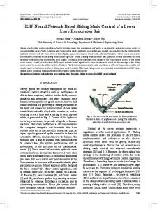
2 Flexible-links modelling Fig. 1 shows the structure of the flexible-link used. Assume that the flexible-link is uniformly elastic and is an EulerBernoulli beam with its torsion and strain set being zero. This assumption is acceptable provided that the strain and torsion are negligible compared with deflection.
Fig. 1: Flexible-link’s structure.
If the flexible-link doesn’t have any deflection, aligns on x1 axis. Deflection of any point of the link at any time presented by w(x,t) and it is derived by solving Euler-Bernoulli beam equation [4]. ∂ 4 W (x, t ) ∂ 2 W (x, t ) + ρA =0 4 ∂x ∂t 2 E : Young' s Modulus
EI
(1)
f si = 0.2 k si ,
A : the Link Cross−Sectional Area I : Inertia of the Link ρ : the Link ' s Density By separating variables, the solution of the equation is given in Equation (2). To satisfy the boundary condition, the final result will be obtained from adding the terms given in Equation (2). In other word, the complete solution of EulerBernoulli equation is given in Equation (3). The natural frequencies of the vibrations are denoted by ωi and they are obtained from Equation (4). The singular vectors {φ1 ,..., φ∞ } are a set of functions that satisfy in Equation (5). w i (x , t ) = φ i (x )δ i (t )
W ( x, t ) =
(2)
∞
∑ φ ( x )δ ( t )
(3)
EI ρ AL4
(4)
i
i
i =1
ωi = βi2
φ i (x ) = c i [(Sinβ i x − Sinhβ i x ) −
(Cosβi x − Coshβi x )]
(Sinβi L + Sinhβi L ) × (Cosβi L + Coshβi L )
(5)
The ci constants normalize these functions such that Equation (6) was satisfied. In fact for measuring deflection finite number of these terms it is assumed (Assumed modes method). This number is dependent on the flexibility of the manipulator and its vibration [4].
∫
L
0
φi (x )2 dx = 1
(6)
( ) ( )
&θ& n1 θ& , δ, δ& + f v + f c u B(δ ) + (7) = && & & δ n 2 θ, δ + K s δ + Fs δ 0 With respect to the above assumptions and by recursive Lagrange approach the dynamic equations are derived in Equation (7). θ is the hub angle, δ is an m×1 vector of deflection variables which m represents the number of assumed modes, n1 and n2 demand the coriolis and centrifuge forces and B is a positive definite symmetric matrix which was known as inertia matrix [4], [8]. n θ& , δ, δ& = 2M θ& Φ T δ Φ T δ&
( ) L ( e )( e ) n 2 (θ& , δ ) = − M L θ& 2 (Φ e Φ e T )δ
diagonal matrix which represents the internal viscose friction of the flexible structure, fc is the coulomb friction was modeled by a sign function but to eliminate discontinuity; the coulomb friction was modeled by Equation (8). Equation (9) defines the end point position [4]. f v = vθ&
1
Φ Te = Φ T |x =L = [φ1 ,..., φ m ] | x =L , φie = φi (x ) |x =L Ks=Diag{ksi,…,ksm} is the stiffness coefficient and it is a positive definite diagonal matrix. fv denotes the viscous friction in the hub position, the structural damping was shown by Fs=Diag{fsi,…,fsm} that is a positive definite
k si = EI
L d 2φ (x) [ i 2 ]2 dx dx 0
∫
1 for θ& > 0 f c = C coulSGN θ& and SGN θ& = − 1 for θ& < 0 0 for θ& = 0 f c = C coul 2−aθ& − 1, C coul > 0 , a > 0 1+ e 1 y t = θ + pδ, p = [φ1 (L ),..., φ m (L )] L
()
()
(8) (9)
3 Physical characteristics of flexible-link Table 1 shows the parameters of a real link where, L is the length of the link, γ is mass per unit of length, I0 denotes the joint actuator inertia and J0 is the link inertia relative to the joint, v represents the hub damping coefficient, Ccoul is the coulomb friction coefficient. E shows the young’s modulus. The inertia momentum of the beam equals I and ωi is the i’th oscillation frequency. The fsi parameters are the structural damping coefficients and ML is the mass of the payload. In this case we have a vibration mode (m=1). The link mass illustrated by mb and the load inertia is given by JL [4], [8]. v Ccoul EI ω1 mb fs1 ML L γ J0 I0 JL
0.59 Nm/rads-1 4.72 Nm for θ& >0 and 4.77 Nm for θ& 0
(14)
κˆ κ ξ − k ⋅ SGN(s ) κˆ κˆ κ = G − k ⋅ SGN(s ) κˆ κ (15) ss& = sG u − k | s |< 0, | G |≤ G u κˆ In this case, G shows the value of uncertainty in system modeling. With respect to the structure of system κκˆ is = −ξ +
positive. To converge the states of the system towards defined surface, (15) must always be satisfied, in which Gu is the highest band of G. If the value of s is negative (15) will be satisfied. By assuming that s is positive and Equation (13) holds, the inequality (17) is obtained [5]. κ (16) υ −1 ≤ ≤ υ κˆ k ≥ υ(G u + χ ) , χ > 0 (17) By choosing this value for k, the goal is achieved. The notable problem in this case is robustness of controller against uncertainty. If disturbances and uncertainties are in the range such that the inequality (17) is satisfied, the closed loop control process is stable and states of the system converge to the desired surface. In spite of these advantages, they have great shortcoming which is high frequency oscillation which can increase the energy and destroy the actuators in a short time. In general, chattering must be eliminated for the controller to perform properly. This can be achieved by smoothing control discontinuity in a thin boundary layer neighboring the switching surface where ψ is the boundary layer thickness as illustrated in Fig. 2. B( t ) = {x, s( x , t ) ≤ ψ} , ψ>0 All trajectories starting inside B(t=0) remain inside B(t) for all t ≥ 0 ; and we then interpolate u inside B(t) and if they
B Fig. 2: Saturation function. By using an adaptive saturation unit, chattering phenomenon will be considerably reduced. (See Fig. 4) In such a manner that the corresponding parameters of the unit may get their desired values adaptively. The required adaptation task is done by a neural network whose outputs are the adjusted parameters of the said unit. The desired nonlinear mapping of the unit may be shown as follows: es − e −s (18) es + e − s Since for the purpose of differentiation, we need continuity property for the unit, we may get the same features by using the continuous version of the saturation block, i.e., a sigmoid function whose main parameters (k, α) are adjusted by a neural network (See Fig. 3). Finally as an important issue, it must be noted that in nonminimum phase systems, the chosen surface takes different dynamics with respect to the input signal and the system may become unstable in response to some particular inputs [6]. u s = k ⋅ tanh(αs) , tanh (s ) =
Fig. 3: Smooth switch used in this paper.
5 Controller modification by neural network By using sigmoid function with constant slew rate of α′ = αk and constant amplitude of k, the chattering was eliminated. By changing these two parameters the suitable
control signal will be accessible. To overcome different uncertainties and external disturbances these parameters should changed manually. Analytically design to find these values will be a difficult procedure and take much more time. Also, unsuitable values will increase consumption energy or make the system unstable. Because of these problems in this section, by applying neural network and defining a cost function like that of (19) and neural network training, the two parameters α and k will be obtained automatically such that the suitable performance of controller will be obtained. Fig. 4 shows the neural network added to control process. 1 J = u s2 (19) 2 For parameter generating a 3-layer neural network is assumed. Also, hidden layer neurons are unipolar and the output layer of network is linear. Error back propagation method was used to train the network only the weights are trained. The training process is online. i = [e u s ]T , o = [α k ]T o h = 1 (1 + exp(−2n h )) , n h = w h i o = n o , n o = w oo h ∆w o = −µ o
∂J ∂ 0 ∂n o ∂o ∂n o ∂w o
∆w h = −µ h
∂J ∂ 0 ∂n o ∂o h ∂n h ∂o ∂n o ∂o h ∂n h ∂w h
The reason of using us in equation (19) is that, the greatest part of oscillation in control signal obtained from this part. The variables which could adjust this part of control signal are k and α. Then the sigmoid slew rate (αk) and maximum amplitude (k) must be adaptively adjusted such that this goal is achieved. It is so important that if neural network entering in control process the stability of the structure is unproved. To initial weighting the Nguyen-Widrow algorithm is used. Also it is possible to employ some other learning methods. But, because the stability of neural network is not proved as such, this method can be employed to control modification process. With respect to the S.M.C. advantages and by reviewing Inequality (17) it was obtained clearly if neural network outputs were diverged such that (17) was satisfied and α was a positive value the system wasn't be unstable.
Path_Generator
S.M.C
Flexible_Link
U
Sliding Mode Controller
N.N
em k alf a
us
Adaptive Saturation Unit
Fig. 4: Applying neural network to control process.
6 Simulations The simulation cases were illustrated in Table 2. Case no. first second third fourth
Uncertainty × √ × √
Adaptation box × × √ √
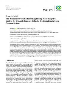
Table 2: simulation cases. By applying discontinuous switch function in S.M.C. the results are verified without uncertainty presence, the chattering problem was clearly observed. But in the first case where sigmoid function with k=2 and α=1 was used the chattering phenomenon was eliminated and less energy was consumed (See Fig. 5). To modify the performance of controller, the neural network is added to the controller structure. In the third case, the rise time increases but the settling time reduces. Fig. 6(a) and Fig. 6(b) show the results of simulations for first case and third case. Fig. 6(c) shows the convergence of α and k. Energy consumption is implemented by Fig. 6(d) for these two cases. By adding 50% uncertainty in coulomb friction modeling, the rise time and the settling time were increased. To improve the controller performance and reduce the rise time value k must be increased. But in this case, the energy consumption also increases. The value of α and k were chosen approximately in the second case (k=4, α=2), and, therefore, the best performance could not be expected. In the second case and fourth case, the observed changes were similar to the previous case. Only in the fourth case will the parameters converge to higher values from third case. The results are shown in Fig. 7. Large absolute value of error causes the parameters increase with a high rate at the beginning of simulations (See figures 6(c) and 7(c)). But when the error came down to zero their values decreased with a high slope. The adaptive performance of the neural network completely is observable here. The difference between consumed energy in the third and fourth cases is shown in figures 6(d) and 7(d). It can be seen in the mentioned figures the consumed energy in the presence of neural network considerably lowers than that of the other case. Again the reason for this phenomenon is the flexibility for adjustment of the parameters k and α. As before noted the parameters converge to higher values in the fourth case. In fact adaptive characteristic of the neural network make the controller performance better. As last point it must be noted that selecting η and λ is very important. Some values of them cause instability in controller or unacceptable transient performance. In terms of asymptotic stability region of the closed loop system one may consider that parameters converge to larger value when there is no neural network.
7 Conclusions The sliding mode controllers show up enough robustness against uncertainty and disturbances. However their important disadvantage is chattering phenomenon and that
smoothing switch function can eliminate it. One of the problems that are to be studied is how to choose a smooth function instead of a switch function. In this approach use of a sigmoid function is usual. Nevertheless, selection of the amplitude and slope of the sigmoid function had been done in different ways. In this paper, a neural network is used to adjust the parameters. So, the controller employs the advantages of neural network (robustness and adaptation). The equivalent control signal depends on system structure and hence, does not vary. It should be noted that the switching part of control signal can be selected such that the best performance is achieved. To achieve better performance while improving the stability, the dynamic switches are recommended.
Systems, Man & Cybernetics, volume 4, pp. 26192624, (2000). H.A. Talebi, R.V. Patel, K. Khorasani, Control of flexible-link manipulators using neural networks, Springer-Verlag, (2001). J. E. Slotine, W. Li. Applied nonlinear control, Prentice-Hall, (1991). K. Barikbin. Control of non-minimum phase uncertain nonlinear systems by adaptive sliding mode, Tehran University, Faculty of Engineering, (2001). M. Gokasan, O. S. Bogosyan, A. Arabyan, A. Sabanovic. “A sliding mode based controller for a flexible arm with a load”, IEEE Industrial Electronics and Control, volume 2, pp. 1083-1087, Aachen, Germany, (1998). M. J. Yazdanpanah, K. Khorasani, R.V. Patel. “Uncertainty compensation for a flexible-link manipulator using nonlinear H∞ control”, International Journal of Control, volume 69, no. 6, pp. 753- 771, (1998). V. Utkin. Sliding modes and their application in variable structure systems, Mir Publishers, Moscow, (1978). V. Utkin, J. Guldner, J. Shi. Sliding mode control in electromechnical systems, Taylor & Francis, (1999).
[4] [5] [6]
[7]
References
[8] A. Piazzi, A. Visioli. “End-point control of a flexible-link via optimal dynamic inversion”, IEEE/ASME International Conference on Advanced Intelligent Mechatronics, pp. 936-941, (2001). D. Karandikar, B. Bandyopadhyay. “Sliding mode [9] control of single link flexible manipulator”, IEEE ICIT Conf., pp. 712-717, (2000). D. K. Wedding, A. H. Eltimsahy. “Flexible Link [10] Control Using Multiple Forward Paths, Multiple RBF Neural Networks in a Direct Control Application”, IEEE International Conference on
[1]
[2] [3]
1.2
6 4
0.8
control effort
endpoint(rad)
1
0.6 0.4
0
0.2 −2
0 −0.2
0
5
10 (a)
15
−4
20
0
5
time(s)
10 (b)
2.5
50
2
40
1.5
energy(J)
control effort
2
1
15
20
15
20
time(s)
30 20
0.5 10
0 −0.5
0
5
10 (c)
15 time(s)
20
0
0
5
10 (d)
time(s)
Fig. 5: Comparison of the simulation results of the end point control between discontinuous and continuous switches. (a)- End point position, discontinuous switch (…), smooth switch (___); (b) - Control signal, discontinuous switch (…) (c)- Control signal, smooth switch (___); (d) - Energy Consumption, discontinuous switch (…), smooth switch (___).
1.2
2.5
1
2 1.5
control effort
endpoint(rad)
0.8 0.6 0.4
1 0.5
0.2
0
0 −0.2
0
5
10
20
−0.5
5
10 (b)
2
4
1.5
3
1
0.5
0
0
time(s)
energy(J)
parameters(k,a)
(a)
15
15
20
15
20
15
20
15
20
time(s)
2
1
0
5
10 (c)
15
0
20
0
5
time(s)
10 (d)
time(s)
Fig. 6: Comparison of the simulation results of the end point control between first case and third case. (a)- End point position; (b) - Control signal, first case (…..) and third case (____); (c)- Convergence of k (___) and α (…..); (d) - Energy Consumption, first case (…..) and (__) third case. 1.2
4 3
0.8
control effort
endpoint(rad)
1
0.6 0.4
2 1
0.2 0
0 −0.2
0
5
10 (a)
15
20
−1
0
5
time(s)
10 (b)
4
time(s)
6
energy(J)
parameters(k,a)
5 3
2
4 3 2
1 1 0
0
5
10 (c)
15 time(s)
20
0
0
5
10 (d)
time(s)
Fig. 7: Comparison of the simulation results of the end point control between second case and fourth case. (a)- End point position; (b) - Control signal, second case (…..) and fourth case (____); (c)- Convergence of k (___) and α (…..); (d) - Energy Consumption, second case (…...) and fourth case (__).