International Journal of Computer Science, Engineering and Information Technology (IJCSEIT), Vol.1, No.5, December 2011
MODIFIED HISTOGRAM EQUALIZATION FOR IMAGE CONTRAST ENHANCEMENT USING PARTICLE SWARM OPTIMIZATION P.Shanmugavadivu1, K.Balasubramanian2 and K.Somasundaram3 1,3
Department of Computer Science and Applications, Gandhigram Rural Institute – Deemed University, Gandhigram, India, 1
[email protected],
[email protected]
2
Department of Computer Applications, PSNA College of Engineering and Technology, Dindigul, India,
[email protected]
ABSTRACT A novel Modified Histogram Equalization (MHE) technique for contrast enhancement is proposed in this paper. This technique modifies the probability density function of an image by introducing constraints prior to the process of histogram equalization (HE). These constraints are formulated using two parameters which are optimized using swarm intelligence. This technique of contrast enhancement takes control over the effect of HE so that it enhances the image without causing any loss to its details. A median adjustment factor is then added to the result to normalize the change in the luminance level after enhancement. This factor suppresses the effect of luminance change due to the presence of outlier pixels. The outlier pixels of highly deviated intensities have greater impact in changing the contrast of an image. This approach provides a convenient and effective way to control the enhancement process, while being adaptive to various types of images. Experimental results show that the proposed technique gives better results in terms of Discrete Entropy and SSIM values than the existing histogram-based equalization methods.
KEYWORDS Contrast Enhancement, Histogram, Histogram Equalization (HE), Probability Density Function (PDF), Cumulative Density Function (CDF), Swarm Intelligence
1. INTRODUCTION Contrast enhancement plays a vital role in image processing for both human and computer vision. It is used as a preprocessing step in medical image processing, texture synthesis, speech recognition and many other image/video processing applications [1] - [3]. Different techniques have already been developed for this purpose. Some of these methods make use of simple linear or nonlinear gray level transformation functions [4] while the rest use complex analysis of different image features such as edge, connected component information and so on.
DOI : 10.5121/ijcseit.2011.1502
13
International Journal of Computer Science, Engineering and Information Technology (IJCSEIT), Vol.1, No.5, December 2011
Histogram is a statistical probability distribution of each gray level in a digital image. The histogram-based equalization techniques are classified into two principal categories as global and local histogram equalization. Global Histogram Equalization (GHE) uses the histogram information of the entire input image in its transformation function. Though this global approach is suitable for overall enhancement, it fails to preserve the local brightness features of the input image. Normally in an image, the high frequency gray levels dominate the low frequency gray levels. In this situation, GHE remaps the gray levels in such a way that the contrast stretching is restricted to some dominating gray levels having larger image histogram components and causes significant contrast loss for the rest of them. Local histogram equalization (LHE) [4] tries to eliminate such problems. It uses a small window that slides through every pixel of the image sequentially. The block of pixels that are masked by the window are considered for HE. Then, the gray level mapping for enhancement is done only for the center pixel of that window. Thus, it makes use of the local information remarkably. However, LHE requires high computational cost and sometimes causes over-enhancement in some portions of the image. Moreover, this technique has the problem of enhancing the noises in the input image along with the image features. The high computational cost of LHE can be minimized using non-overlapping block based HE. Nonetheless, these methods produce an undesirable checkerboard effects on enhanced images. Histogram Equalization (HE) is a very popular technique for contrast enhancement of images [1] which is widely used due to its simplicity and is comparatively effective on almost all types of images. HE transforms the gray levels of the image, based on the probability distribution of the input gray levels. Histogram Specification (HS) [4] is an enhancement technique in which the expected output of image histogram can be controlled by specifying the desired output histogram. However, specifying the output histogram pattern is not a simple task as it varies with images. A method called Dynamic Histogram Specification (DHS) [5] generates the specified histogram dynamically from the input image. Though this method preserves the original input image histogram characteristics, the degree of enhancement is not significant. Brightness preserving Bi-Histogram Equalization (BBHE) [6], Dualistic Sub-Image Histogram Equalization (DSIHE) [7] and Minimum Mean Brightness Error Bi-Histogram Equalization (MMBEBHE) [8] are the variants of HE based contrast enhancement. BBHE divides the input image histogram into two parts, based on the mean brightness of the image and then each part is equalized independently. This method tries to overcome the problem of brightness preservation. DSIHE method uses entropy value for histogram separation. MMBEBHE is an extension of BBHE method that provides maximal brightness preservation. Though these methods can perform good contrast enhancement, they also cause annoying side effects depending on the variation of gray level distribution in the histogram. Recursive Mean-Separate Histogram Equalization (RMSHE) [9], [10], Recursive Sub-image Histogram Equalization (RSIHE) [11] and Recursively Separated and Weighted Histogram Equalization (RSWHE) [12] are the improved versions of BBHE. However, they are also not free from side effects. To achieve sharpness in images, a method called Sub-Regions Histogram Equalization (SRHE) is recently proposed [13] in which the image is partitioned based on the smoothed intensity values, obtained by convolving the input image with Gaussian filter. In this paper, we propose a Modified Histogram Equalization (MHE) method by extending Weighted Thresholded HE (WTHE) [14] 14
International Journal of Computer Science, Engineering and Information Technology (IJCSEIT), Vol.1, No.5, December 2011
method for contrast enhancement. In order to obtain the optimized weighing constraints, Particle Swarm Optimization (PSO) [16] is employed. Section 2 discusses the popular HE techniques. In section 3, the principle of the proposed method is presented. Section 4 presents the information about two widely used statistical techniques to assess image quality. The basic principle of PSO and the procedure to obtain optimized weighing constraints using PSO are described in section 5. The results and discussions are given in section 6 and in section 7 the conclusion is given.
2. HE TECHNIQUES In this section, the existing HE approaches such as GHE, LHE, various partition based HE methods and WTHE are reviewed briefly.
2.1. Global Histogram Equalization (GHE) For an input image F(x, y) composed of discrete gray levels in the dynamic range of [0,L-1], the transformation function C(rk) is defined as: k
∑
S k = C ( rk ) =
i=0
k
P ( ri ) =
∑ i=0
ni n
(1)
where 0 ≤ Sk ≤ 1 and k = 0, 1, 2, …, L-1, ni represents the number of pixels having gray level ri , n is the total number of pixels in the input image and P(ri) represents the Probability Density Function of the input gray level ri. Based on the PDF, the Cumulative Density Function is defined as C(rk). The mapping given in equation (1) is called Global Histogram Equalization or Histogram Linearization. Here, Sk is mapped to the dynamic range of [0, L-1] by multiplying it with (L-1). Using the CDF values, histogram equalization maps an input level k into an output level Hk using the level-mapping equation:
H k = ( L − 1) × C ( rk )
(2)
For the traditional GHE described above, the increment in the output level Hk is given by:
∆ H k = H k − H k −1 = ( L − 1) × P ( rk )
(3)
The increment of level Hk is proportional to the probability of its corresponding level k in the original image. For images with continuous intensity levels and PDFs, such a mapping scheme would perfectly equalize the histogram in theory. However, the intensity levels and PDF of a digital image are discrete in practice. In such a case, the traditional HE mapping is not ideal and it results in undesirable effects where the intensity levels with high probabilities often become overenhanced and the levels with low probabilities get less enhanced and their frequencies get either reduced or even eliminated in the resultant image. 15
International Journal of Computer Science, Engineering and Information Technology (IJCSEIT), Vol.1, No.5, December 2011
2.2. Local Histogram Equalization (LHE) Local Histogram Equalization (LHE) performs block-overlapped histogram equalization. LHE defines a sub-block and retrieves its histogram information. Then, histogram equalization is applied at the center pixel using the CDF of that sub-block. Next, the window is moved by one pixel and sub-block histogram equalization is repeated until the end of the input image is reached. Though LHE cannot adapt to partial light information, it still over-enhances certain portions depending on its window size. However, selection of an optimal block size that enhances all parts of an image is not an easy task to perform.
2.3. Histogram Partitioning Approaches BBHE tries to preserve the average brightness of the image by separating the input image histogram into two parts based on the input mean and then equalizing each of the parts independently. RMSHE, RSIHE and RSWHE partition the histogram recursively. Here, some portions of histogram among the partitions cannot be expanded much, while the outside region expands significantly that creates unwanted artifacts. This is a common drawback of most of the existing histogram partitioning techniques since they keep the partitioning point fixed throughout the entire process of equalization. In all the recursive partitioning techniques, it is not an easy job to fix the optimal recursion level. Moreover, as the recursion level increases, recursive histogram equalization techniques produce the results same as GHE and it leads to computational complexity.
2.4. Weighted Thresholded HE (WTHE) WTHE is a fast and efficient method for image contrast enhancement [14]. This technique provides a novel mechanism to control the enhancement process, while being adaptive to various types of images. WTHE method provides a good trade-off between the two features: adaptivity to different images and ease of control, which are difficult to achieve in GHE-based enhancement methods. In this method, the probability density function of an image is modified by weighting and thresholding prior to HE. A mean adjustment factor is then added with the expectation to normalize the luminance changes. But, while taking the mean of the input and reconstructed images, the highly deviated intensity valued pixels known as outlier pixels are also taken into account. This will not effectively control the luminance change in the output image, which is a major drawback of this method. The outlier pixels are the pixels which are usually less in number and are having distant intensity values than the other pixels.
3. MODIFIED HISTOGRAM EQUALIZATION (MHE) The proposed method, MHE is an extension of WTHE which performs histogram equalization based on a modified histogram. Each original probability density value P(rk) is replaced by a Constrained PDF value Pc(rk) yielding:
∆ H k = ( L − 1) × Pc ( rk )
(4)
16
International Journal of Computer Science, Engineering and Information Technology (IJCSEIT), Vol.1, No.5, December 2011
The proposed level mapping algorithm is given below. Step 1: Input the image F(i, j) with a total number of ‘n’ pixels in the gray level range 1] Step 2: Compute the Probability Density Function (PDF), P(rk) for the gray levels Step 3: Find the median value of the PDFs, M1 Step 4: Compute the upper constraint ‘Pu’ : Pu = v * max(PDF) where 0.1 < v < 1.0 Step 5: Set power factor ‘r’ where 0.1 < r < 1.0 Step 6: Set lower constraint factor Pl be as low as 0.0001 Step 7: Compute the constrained PDF, Pc (rk )
[0,L-
Pc ( rk ) = T ( P ( rk )) Pu P ( rk ) − Pl = Pu − Pl 0
if Pl < P ( rk ) ≤ Pu if P ( rk ) ≤ Pl if P ( rk ) > Pu
r
* Pu
(5)
Step 8: Find the median value of the constrained PDFs, M2 Step 9: Compute the median adjustment factor Mf as: Mf = M2 – M1 Step 10: Add Mf to the constrained PDFs Step 11: Compute cumulative probability density function, Cc(F(i,j)) Step 12: Apply the HE procedure (level mapping) as:
F ′( i , j ) = ( L − 1) × C c ( F ( i , j ))
(6)
where F′(i, j) is the enhanced image The transformation function T(.) in equation (5) transforms all the original PDF values between the upper constraint Pu and the lower constraint Pl using a normalized power law function with index r > 0. In this level-mapping algorithm, the increment for each intensity level is decided by the transformed histogram given in equation (5). The increment is controlled by adjusting the index r of the power law transformation function. For example, when r < 1, the power law function gives a higher weightage to the low probabilities. Therefore, the lower probability levels are preserved and the possibility of over-enhancement is less. The effect of the proposed method approaches that of the GHE, when r→1. When r > 1, more weight is shifted to the high-probability levels and MHE would yield even stronger effect than the traditional HE. The upper constraint Pu is used to avoid the dominance of the levels with high probabilities when allocating the output dynamic range. The lower constraint Pl is used to find the levels whose probabilities are too low. The Pl value is set to be as low as 0.0001. Any pixel having its probability less than the lower constraint Pl is having very low impact in the process of contrast 17
International Journal of Computer Science, Engineering and Information Technology (IJCSEIT), Vol.1, No.5, December 2011
enhancement. It can be observed from equation (5) that when r = 1, Pu=1 and Pl = 0, the proposed MHE reduces to GHE. After the constrained PDF is obtained from equation (5), the median adjustment factor (Mf) is calculated by finding the difference between the median value of the constrained PDFs and the median value of the original PDFs. Then, the Mf is added to the constrained PDFs which will effectively control the luminance change, since the outlier pixels are ignored while computing the medians. The cumulative density function (CDF) is obtained as: k
C c (k ) =
∑ P ( m ), c
for k = 0 ,1,..., L − 1
(7)
m =0
Then, the HE procedure is applied as given in equation (6). This will not cause serious level saturation (clipping), to the resulting contrast enhanced image. The two important parameters namely, v and r, used in this algorithm play a vital role in enhancing the contrast. Both v and r are accepting values in the range from 0.1 to 1.0. In order to find the optimum values for v and r, particle swarm optimization technique is employed in which an objective function is defined which will maximize the contrast of an input image. There are several measures such as Structural Similarity Index Matrix (SSIM) [11], Discrete Entropy (DE) [15] etc which are used to calculate the degree of image contrast enhancement. One such measure can be considered to be an objective function. In this paper, it is found that DE is providing better trade-off than SSIM. Hence, DE has been selected as an objective function. SSIM is used as a supporting comparative measure.
4. METRICS TO ASSESS IMAGE QUALITY 4.1. Structural Similarity Index Matrix (SSIM) The Structural Similarity Index Matrix (SSIM) is defined as: SSIM ( X , Y ) =
( 2 µ X µ Y + C1 )(2σ XY + C 2 )
(8)
( µ X2 + µ Y2 + C1 )(σ X2 + σ Y2 + C 2 )
where X and Y are the reference and the output images respectively; µ X and µ Y are respective mean of X and Y, σ X and σ Y are the standard deviation of X and Y respectively, σ XY is the square root of covariance of X and Y, whereas C1 and C2 are constants. The SSIM value between two images X and Y is generally in the range 0 to 1. If X=Y, then the SSIM is equal to 1 which implies that when the SSIM value is nearing 1, the degree of structural similarity between the two images are more. 18
International Journal of Computer Science, Engineering and Information Technology (IJCSEIT), Vol.1, No.5, December 2011
4.2 Discrete Entropy (DE) Discrete entropy E(X) measures the richness of details in an image after enhancement. It is defined as: 255
E ( X ) = − ∑ p ( X k ) log 2 ( p ( X k ))
(9)
k =0
The details of the original input image is said to be preserved in the enhanced image is said to be preserved in the enhanced image, when the entropy value of the latter is closer to that of the former.
5. PARTICLE SWARM OPTIMIZATION (PSO) In the proposed technique, PSO is adopted to find optimal values of ‘v’ and ‘r’. PSO was first proposed by Eberhart and Kennedy [16]. This technique is a population-based optimization algorithm. It uses a number of agents (particles) that constitute a swarm moving around in the search space looking for the best solution. Each particle keeps track of its coordinates in the solution space which are associated with the best solution (fitness) that has achieved so far by that particle. This value is called personal best, pbest and another best value that is tracked by the PSO is the best value obtained so far by any particle in the neighbourhood of that particle, is called global best, gbest. The basic concept of PSO lies in accelerating each particle towards its pbest and the gbest locations, with a random weighted accelaration at each time as shown in Fig. 1.
Figure 1. Modification of a searching point by PSO Sk Sk+1 Vk Vk+1 Vpbest Vgbest
: current searching point : modified searching point : current velocity : modified velocity : velocity based on pbest : velocity based on gbest
19
International Journal of Computer Science, Engineering and Information Technology (IJCSEIT), Vol.1, No.5, December 2011
Each particle tries to modify its position using the following information: the current position, the current velocity, the distance between the current position and pbest, the distance between the current position and the gbest. Each particle’s velocity can be modified using the equation (10). Vi
k +1
k
k
k
= wVi + c1 × rand () × ( pbesti − s i ) + c 2 × rand () × ( gbesti − si )
(10)
where, vik is the velocity of agent i at iteration k (usually in the range, 0.1- 0.9); c1 and c2 are the learning factors in the range, 0 - 4; rand() is the uniformly distributed random number between 0 and 1; sik is the current position of agent i at kth iteration; pbesti is present best of agent i and gbest is global best of the group. w, the inertia weight is set to be in the range, 0.1 - 0.9 and is computed as:
w=
wMax − [(wMax − wMin) × iteration] max Iteration
(11)
Using the modified velocity, the particle’s position can be updated as:
Si
k +1
k
= S i + Vi
k +1
(12)
The optimal values of v and r are found using the following procedure: Step 1: Initialize particles with random position and velocity vector Step 2: Loop until maximum iteration Step 2.1: Loop until the particles exhaust Step 2.1.1: Evaluate the difference between Discrete Entropy values of original and MHEed image (p) Step 2.1.2: If p