Module Checking of Strategic Ability - CiteSeerX

Module Checking of Strategic Ability Wojciech Jamroga

Aniello Murano

Institute of Computer Science Polish Academy of Sciences

Dipartimento di Ingegneria Elettrica e Tecnologie dell’Informazione Università degli Studi di Napoli Federico II, Italy

[email protected]

ABSTRACT Module checking is a decision problem proposed in late 1990s to formalize verification of open systems, i.e., systems that must adapt their behavior to the input they receive from the environment. It was recently shown that module checking offers a distinctly different perspective from the betterknown problem of model checking. So far, specifications in temporal logic CTL have been used for module checking. In this paper, we extend module checking to handle specifications in alternating-time temporal logic (ATL). We define the semantics of ATL module checking, and show that its expressivity strictly extends that of CTL module checking, as well as that of ATL itself. At the same time, we show that ATL module checking enjoys the same computational complexity as CTL module checking. We also investigate a variant of ATL module checking where the environment acts under uncertainty. Finally, we revisit the semantics of ability in the module checking problem, and propose a variant where strategies of agents in the module depend only on what the agents are able to observe.

Categories and Subject Descriptors I.2.11 [Artificial Intelligence]: Distributed Artificial Intelligence—Multiagent Systems; I.2.4 [Artificial Intelligence]: Knowledge Representation Formalisms and Methods—Modal logic

General Terms Theory, Verification

Keywords Module checking, model checking, verification, alternatingtime logic, strategic behavior

1.

INTRODUCTION

Model checking is a well-established formal method to automatically check for global correctness of systems [10, 33]. In order to verify whether a system is correct with respect to a desired property, we describe its structure with a mathematical model, specify the property with a logical formula, Appears in: Proceedings of the 14th International Conference on Autonomous Agents and Multiagent Systems (AAMAS 2015), Bordini, Elkind, Weiss, Yolum (eds.), May 4–8, 2015, Istanbul, Turkey. c 2015, International Foundation for Autonomous Agents Copyright and Multiagent Systems (www.ifaamas.org). All rights reserved.

[email protected]

and check formally if the model satisfies the formula. Model checking was first proposed for analysis of closed systems whose behavior is completely determined by their internal states and transitions. In this setting, models are often given as state transition graphs that usually include some degree of internal nondeterminism. An unwinding of the graph results in an infinite tree, formally called computation tree, that collects all possible evolutions of the system. Model checking of a closed system amounts to checking whether the tree satisfies the logical specification. Properties for model checking are usually specified in temporal logics CTL, LTL, CTL* [14], or strategic logics ATL, ATL* [2, 3]. In module checking [22, 25], the system is modeled as a module that interacts with its environment, and correctness means that a desired property must hold with respect to all possible interactions. The module can be seen as a transition system with states partitioned into ones controlled by the system and by the environment. Notice that the environment represents an external additional source of nondeterminism, because at each state controlled by the environment the computation can continue with any subset of its possible successor states. In other words, while in model checking we have only one computation tree to check, in module checking we have an infinite number of trees to handle, one for each possible behavior of the environment. Properties for module checking are usually given in CTL or CTL*. It was believed for a long time that module checking of CTL/CTL* is a special (and rather simplistic) case of model checking ATL/ATL*. Because of that, active research on module checking subsided shortly after its conception. The belief has been recently refuted in [20]. There, it was proved that module checking includes two features inherently absent in the semantics of ATL, namely irrevocability and nondeterminism of strategies. This made module checking an interesting formalism for verification of open systems again. In this paper, we extend module checking to handle specifications in the more expressive logic ATL. We define the semantics of ATL module checking, and show that its expressivity strictly extends that of CTL module checking, as well as that of ATL itself. At the same time, we show that ATL module checking enjoys the same computational complexity as CTL module checking. We also investigate a variant of ATL module checking where the environment acts under uncertainty, and show – again – that the computational price to pay is not high. Finally, we discuss the semantics of ability in the module checking problem. It turns out that the irrevocability of environment’s strategies may yield counterintuitive interpretation of what agents can enforce. To deal

with it, we propose a variant where strategies of agents in the module cannot depend on the whole strategy of the environment, but only on what the agents have so far observed. Related work. Module checking was introduced in [22, 25], and later extended in several directions. In [23], the basic CTL/CTL* module checking problem was extended to the setting where the environment has imperfect information about the state of the system. In [8], it was extended to infinite-state open systems by considering pushdown modules. The pushdown module checking problem was first investigated for perfect information, and later, in [5, 7], for imperfect information; the latter variant was proved undecidable in [5]. [15, 4] extended module checking to µ-calculus specifications, and in [32] the module checking problem was investigated for bounded pushdown modules (or hierarchical modules). From a more practical point of view, [28, 29] built a semi-automated tool for module checking in the existential fragment of CTL, both in the perfect and imperfect information setting. Moreover, an approach to CTL module checking based on tableau was exploited in [6]. Finally, an extension of module checking was used to reason about three-valued abstractions in [17, 11, 18, 16]. It must be noted that literature on module checking became rather sparse after 2002, especially when compared to the body of work on model checking. This must be partially attributed to the popular belief that CTL module checking is nothing but a special case of ATL model checking. The belief has been refuted only recently [20], which will hopefully spark renewed interest in verification of open systems by module checking.

2. 2.1

PRELIMINARIES Models and Modules

In this paper, we consider several frameworks for modeling and verification of temporal properties. Modules in module checking [22] were proposed to represent open systems – that is, systems that interact with an environment whose behavior cannot be determined in advance. In their simplest form, modules are unlabeled transition systems with the set of states partitioned into those “owned” by the system, and the ones where the next transition is controlled by the environment. Models of alternating-time temporal logic [3], called concurrent game structures, are multi-player transition systems with transitions labeled by tuples of actions, one from each agent. Definition 1 (Module). A module is a tuple M = hAP, Sts , Ste , q0 , →, PV i, where AP is a finite set of (atomic) propositions, St = Sts ∪Ste is a nonempty finite set of states partitioned into a set Sts of system states and a set Ste of environment states, →⊆ St × St is a (global) transition relation, q0 ∈ St is an initial state, and PV : St → 2AP maps each state q to the set of atomic propositions true in q. Definition 2 (CGS). A concurrent game structure is a tuple M = hAP, Agt, St, Act, d, o, PV i including nonempty finite set of propositions AP , agents Agt = {1, . . . , k}, states St, (atomic) actions Act, and a propositional valuation PV : St → 2AP . The function d : Agt × St → 2Act defines nonempty sets of actions available to agents at each state, and the (deterministic) transition function o assigns the outcome state q 0 = o(q, α1 , . . . , αk ) to each state q and tuple of actions αi ∈ d(i, q) that can be executed by Agt in q.

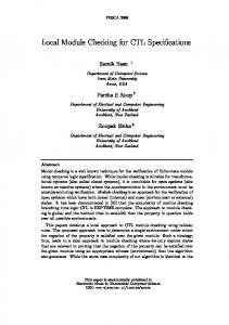
choice qc

black

qb

qw

white

Figure 1: Coffee machine Mcaf . Environment states are marked grey; system states are marked white. A pointed CGS is a pair (M, q0 ) of a concurrent game structure and an initial state in it. Nondeterministic choices of agents in a CGS can be represented by sets of actions. In this sense, agent a can select at state q any nonempty set α ⊆ d(a, q), and the set of successors of α is simply the union of successor sets for each action in α. Then, modules can be seen as a subclass of concurrent game structures – more precisely, 2-player turn-based1 pointed CGS’s with agents Agt = {sys, env}. Example 1. Consider a coffee machine that allows customers to choose between ordering black or white coffee. After the selection, the machine delivers the product and waits for further selections, cf. Figure 1. The environment represents all possible infinite lines of customers, each with their own plans and preferences. We formally define the coffee machine as a module Mcaf = hAP, Sts , Ste , q0 , →, PV i such that AP = {choice, black, white}, Sts = {qb , qw }, Ste = {qc }, q0 = qc , →= {(qc , qb ), (qc , qw ), (qb , qc ), (qw , qc )}, and PV (black) = {qb }, PV (white) = {qw }, PV (choice) = {qc }. We leave rewriting Mcaf as a CGS to the reader.

2.2

CTL Module Checking

CTL* is a branching–time temporal logic [12], where path quantifiers, E (“for some path”) and A (“for all paths”), can be followed by an arbitrary linear-time formula, allowing boolean combinations and nesting over temporal operators X (“next”), U (“strong until”), F (“eventually”), and G (“always”). There are two types of formulas in CTL*: state formulas ϕ, whose satisfaction is related to a specific state (or node of a labeled tree), and path formulas γ, whose satisfaction is related to a specific path. Formally: ϕ ::= p | ¬ϕ | ϕ ∧ ϕ | Eγ, γ ::= ϕ | ¬γ | γ ∧ γ | Xγ | γ U γ. where p is an atomic proposition. The other operators can be defined as: Aγ ≡ ¬E¬γ, Fγ ≡ true U γ, and Gγ ≡ ¬F¬γ. CTL [10] is a restricted subset of CTL*, obtained replacing the syntax of path formulas γ as follows: γ := Xϕ | ϕ U ϕ | ϕ W ϕ (“weak until”), i.e., every path quantifier must be immediately followed by a temporal operator. We define the semantics of CTL* (and its fragment CTL) with respect to a St-labeled tree hT, V i with propositional valuation PV .2 Let x ∈ T and λ ⊆ T be a path from x. 1

A CGS is turn-based iff every state in it is controlled by (at most) one agent. That is, for every q ∈ St, there is an agent a ∈ Agt such that |d(a0 , q)| = 1 for all a0 6= a. 2 For the formal definition of labeled trees, cf. e.g. [22, 20].

By λ[i] we denote the i-st element of λ and by λ[1..∞] the suffix of λ starting at λ[1]. For a state (resp., path) formula ϕ (resp. γ), the satisfaction relation hT, V i, PV , x |=CTL ϕ (resp., hT, V i, PV , λ |=CTL γ) is defined as follows:

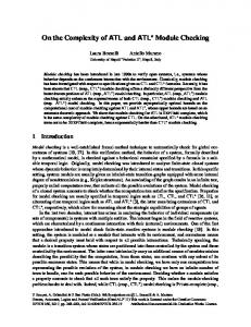
y,∗ se stae,clo v mo

move,open

q1

clean1

q2 move,open

mo stay ve, ,∗ clo se

clean2

• hT, V i, PV , x |=CTL p iff p ∈ PV (x); • hT, V i, PV , x |=CTL Eγ iff there exists a path λ from x such that hT, V i, PV , λ |=CTL γ;

Figure 2: Vacuum cleaner vs. gate controller: Mclean

• hT, V i, PV , λ |=CTL ϕ iff hT, V i, PV , λ[0] |=CTL ϕ; • hT, V i, PV , λ |=CTL Xγ iff hT, V i, PV, λ[1..∞] |=CTL γ; • hT, V i, PV , λ |=CTL γ1 U γ2 iff there is y ∈ λ such that hT, V i, PV , λy |=CTL γ2 and hT, V i, PV , λz |=CTL γ1 for all z ∈ λ such that z ≺ y. The clauses for negation and conjunction are standard. Moreover, hT, V i, PV , λ |=CTL γ1 W γ2 iff either hT, V i, PV , λ |=CTL γ1 U γ2 or hT, V i, PV , λ |=CTL Gγ1 . Given a formula ϕ, we say that hT, V i satisfies ϕ if hT, V i, PV , ε |=CTL ϕ. For a module M = hAP, Sts , Ste , →, q0 , PV i, the set of all (maximal) computations of M starting from the initial state q0 is described by a St-labeled tree hTM , VM i, called computation tree, which is obtained by unwinding M from the initial state in the usual way. The problem of deciding, for a given branching-time formula ϕ over AP , whether hTM , PV ◦VM i 3 satisfies ϕ, denoted M |=CTL ϕ, is the usual model-checking problem [10, 33]. On the other hand, for an open system, hTM , VM i corresponds to a very specific environment, i.e. the maximal environment that never restricts the set of its next states. When we examine specification ϕ w.r.t. a module M , the formula ϕ should hold not only in hTM , VM i, but in all the trees obtained by pruning some environment transitions from hTM , VM i. The set of these trees is denoted by exec(M ) and is formally defined as follows. For each state q ∈ St, let succ(q) be the ordered tuple of q 0 node successors of q, i.e., q → q 0 . A tree hT, V i is in exec(M ) iff T ⊆ TM , V is the restriction of VM to the tree T , and for all x ∈ T the following holds: • if VM (x) = w ∈ Sts and succ(q) = hq1 , . . . , qn i, then children(T, x) = {x · 1, . . . , x · n} (note that for 1 ≤ i ≤ n, V (x · i) = VM (x · i) = qi ); • if VM (x) = w ∈ Ste and succ(q) = hq1 , . . . , qn i, then there is a sub-tuple hqi1 , . . . , qip i of succ(q) such that children(T, x) = {x · i1 , . . . , x · ip } (note that for 1 ≤ j ≤ p, V (x · ij ) = VM (x · ij ) = qij ). Intuitively, when the module M is in a system state qs , then all states in succ(qs ) are possible successors. When M is in an environment state qe , then the possible next states (that are in succ(qe )) depend on the current environment. Since the behavior of the environment is nondeterministic, we have to consider all the nonempty sub-tuples of succ(qe ). For a module M and a CTL(*) formula ϕ, we say that M reactively satisfies ϕ, denoted by M |=rCTL ϕ, if all the trees in exec(M ) satisfy ϕ. The problem of deciding whether M reactively satisfies ϕ is called module checking [25]. Note that M |=rCTL ϕ implies M |=CTL ϕ (since hTM , VM i ∈ exec(M )), but the converse in general does not hold. Also, note that M 6|=rCTL ϕ is not equivalent to M |=rCTL ¬ϕ. 3

PV ◦ VM denotes the composition of the functions PV and VM that allows to re-label each state-labeled node u in hTM , VM i with PV (VM (u)).

Example 2. Consider the coffee machine from Example 1. Clearly, Mcaf |=CTL EFblack as it is (in principle) possible to deliver black coffee. On the other hand, Mcaf 6|=rCTL EFblack. Think of a line of customers who never order black coffee. It corresponds to an execution tree of Mcaf with no node labeled with black, and such a tree does not satisfy EFblack.

2.3

Alternating Time Logic ATL/ATL*

Alternating-time temporal logic [3] generalizes CTL* by replacing path quantifiers E, A with strategic modalities hhAii. Informally, hhAiiγ expresses that the group of agents A has a collective strategy to enforce temporal property γ. The language ATL* is given by the grammar below: ϕ ::= p | ¬ϕ | ϕ ∧ ϕ | hhAiiγ, γ ::= ϕ | ¬γ | γ ∧ γ | Xγ | γ U γ. where A ⊆ Agt is any subset of agents, and p is a proposition. “Sometime” and “always” are obtained like in CTL*. Also, we can use [[A]]γ ≡ ¬hhAii¬γ to express that no strategy of A can prevent property γ. Similarly to CTL, ATL is the syntactic variant in which every occurrence of a strategic modality is immediately followed by a temporal operator. Given a CGS, we define the strategies and their outcomes as follows. A perfect recall strategy for agent a is a function sa : St+ → Act such that sa (q0 q1 . . . qn ) ∈ d(a, qn ). A memoryless strategy for a is a function sa : St → Act such that sa (q) ∈ d(a, q). A collective strategy for a group of agents A = {a1 , . . . , ar } is simply a tuple of individual strategies sA = hsa1 , . . . , sar i. The “outcome” function out(q, sA ) returns the set of all paths that can occur when agents A execute strategy sA from state q on. The semantics |=ATL of alternating-time logic is obtained from that of CTL* by replacing the clause for Eγ as follows: M, q |=ATL hhAiiγ iff there is a perfect recall strategy sA for A such that for every λ ∈ out(q, sA ) we have M, λ |=ATL γ. The problem of deciding whether a pointed CGS (M, q0 ) satisfies the ATL formula ϕ is called ATL model checking. Example 3. A vacuum cleaner robot can move between (and clean) two cubicles, while a controller can open/close the gate between the cubicles. A simple CGS modeling the scenario is depicted in Figure 2. The wildcard (∗) stands for any action of the respective agent. We assume q1 to be the initial state. Clearly, Mclean |=ATL hhrobot, ctrliiFclean1 and Mclean |=ATL hhrobot, ctrliiFclean2 : if the robot and the controller cooperate, they can get any room cleaned. On the other hand, the robot cannot clean the other cubicle on its own, e.g., Mclean 6|=ATL clean1 → hhrobotiiFclean2 . Actually, the controller has a sure strategy to prevent that (by never opening

choice (-,,-)

(,ig n, -) (r eq b, -,)

∗) n, ,ig ) (-,w, eq (r

(-,,-)

qc

qrb

qrw

qer error ilk) r,m pou , (

(-,pour,-)

(-,pour,-)

qb

(-,-,-)

(-,-,ign)

qpr

(-,-,milk)

black

qw white

Figure 3: Multi-agent coffee machine Mcaf2 the gate): Mclean |=ATL clean1 → hhctrliiG¬clean2 . The robot can also prevent cleaning the other room, by never deciding to move: Mclean |=ATL clean1 → hhrobotiiG¬clean2 . Embedding CTL* in ATL*. The path quantifiers of CTL* can be expressed in the standard semantics of ATL* as follows [3]: Aγ ≡ hh∅iiγ and Eγ ≡ hhAgtiiγ. We point out that the above translation of E does not work for several extensions of ATL*, e.g., with imperfect information, nondeterministic strategies, and irrevocable strategies. On the other hand, the translation of A into hh∅ii does work for all the semantic variants of ATL* considered in this paper. Thanks to that, we can define a translation atl(ϕ) from CTL* to ATL* as follows. First, we convert ϕ so that it only includes universal path quantifiers, and then replace every occurrence of A with hh∅ii. For example, atl(EG(p1 ∧ AFp2 )) = ¬hh∅iiF(¬p1 ∨ ¬hh∅iiFp2 ). Note that if ϕ is a CTL formula then atl(ϕ) is a formula of ATL. By a slight abuse of notation, we will use path quantifiers A, E in ATL formulae whenever it is convenient.

3.

ATL MODULE CHECKING

We are now ready to propose how module checking for ATL specifications can be defined.

3.1

Multi-Agent Modules

Definition 3 (Multi-agent module). A multi-agent module is a pointed concurrent game structure that contains a special agent called “the environment” (env ∈ Agt). We call a module k-agent if it consists of k agents plus the environment (i.e., the underlying CGS contains k + 1 agents). The module is alternating iff its states are partitioned into those owned by the environment (i.e., |d(a, q)| = 1 for all a 6= env) and those where the environment is passive (i.e., |d(env, q)| = 1). That is, it alternates between the agents’ and the environment’s moves. Moreover, the module is turnbased iff the underlying CGS is turn-based. We remark in passing that the original modules [22] were turn-based (and hence also alternating). On the other hand, the version of module checking for imperfect information [23] assumed that the system and the environment can act simultaneously.

Example 4. A multi-agent refinement of the coffee machine is presented in Figure 3. The module includes two agents: the brewer (br) and the milk provider (milky). The brewer’s function is to pour coffee into the cup (action pour), and the milk provider can add milk on top (action milk). Moreover, each of them can be faulty and ignore the request from the environment (ign). Note that if br and milky try to pour coffee and milk at the same time, the machine gets jammed and needs repair. Finally, the environment has actions reqb, reqw available in state qc , meaning that it requests black (resp. white) coffee. Since the module is alternating, we have kept the convention of marking system states as white, and environment states as grey.

3.2

Multi-Agent Module Checking

We define the ATL module checking problem analogously to CTL module checking. Given a multi-agent module M and an ATL* formula ϕ, we say that M reactively satisfies ϕ, denoted M |=rATL ϕ, if all the trees in exec(M ) satisfy ϕ. Similarly to CTL, M |=rATL ϕ implies M |=ATL ϕ (since hTM , VM i ∈ exec(M ) and hTM , VM i is strategically bisimilar to M [1]), but the converse in general does not hold. Again, note that M 6|=rATL ϕ is not equivalent to M |=rATL ¬ϕ. Example 5. What questions can be answered with ATL module checking? Consider the multi-agent coffee machine Mcaf2 from Example 4. Clearly, Mcaf2 6|=rATL hhbr, milkyiiFwhite because the environment can keep requesting black coffee. On the other hand, Mcaf2 |=rATL hhbr, milkyiiFblack: the agents can provide the user with black coffee whatever she requests. They can also deprive the user of coffee completely – in fact, the brewer alone can do it by consistently ignoring her requests: Mcaf2 |=rATL hhbriiG(¬black ∧ ¬white). All the above formulae can be also be used for model checking, and they would actually generate the same answers. So, what’s the benefit of module checking? In module checking, we can condition the property to be achieved on the behavior of the environment. For instance, users who never order white coffee can be served by the brewer alone: Mcaf2 |=rATL AG¬reqw → hhbriiFblack. Note that the same formula in model checking does not express any interesting property. In fact, it trivially holds since Mcaf2 6|=ATL AG¬reqw. Likewise, we have Mcaf2 |=ATL AG¬reqb → hhbriiFwhite, whereas module checking gives a different and more intuitive answer: Mcaf2 6|=rATL AG¬reqb → hhbriiFwhite. That is, the brewer cannot handle requests for white coffee on his own, even if the user never orders anything else. More realistic examples can include a group of software agents serving customers on behalf of an online shop (each agent dealing with different merchandise), or a sensor network reacting to the stream of traffic data. We leave formal treatment of the examples to the reader’s imagination.

4.

EXPRESSIVE POWER OF ATL MODULE CHECKING

In this section, we show that ATL module checking strictly enhances the expressivity of both CTL module checking and ATL model checking.

4.1

ATL vs. CTL Module Checking

First, we prove that function atl(ϕ) presented in Section 2.3 provides a sufficient syntactic translation to embed CTL module checking.

Theorem 1. For every module M and CTL* formula ϕ, we have M |=rCTL ϕ iff M |=rATL atl(ϕ). Proof. M |=rCTL ϕ iff for every T ∈ exec(M ) it holds that T |=CTL ϕ. Thus, equivalently, ∀T ∈ exec(M ) . T |=ATL atl(ϕ). But this is equivalent to M |=rATL atl(ϕ). Note that, for a CTL formula ϕ, we have that atl(ϕ) is a formula of ATL. Thus, Theorem 1 provides also an embedding of module checking for “CTL without star.” The next theorem shows that there is no embedding the other way. Theorem 2. There exists a pair of multi-agent modules M1 , M2 that reactively satisfy the same formulae of CTL* (and hence also CTL), but are reactively distinguished by a formula of ATL (and hence also ATL*). Proof. Take M1 = Mcaf2 and M2 identical to M1 except that state qrb is controlled by milky. Now, observe that env has the same “pruning strategies” in M1 , M2 , and that they yield bisimilar subtrees. More formally, for every T1 ∈ exec(M1 ) there is bisimilar T2 ∈ exec(M2 ), and vice versa. Thus, M1 |=rCTL ϕ iff ∀T ∈ exec(M1 ) . T |=CTL ϕ iff ∀T ∈ exec(M2 ) . T |=CTL ϕ iff M2 |=rCTL ϕ. Furthermore, take ϕ ≡ hhmilkyiiG(¬black ∧ ¬white). It is easy to see that M1 6|=rATL ϕ but M2 |=rATL ϕ.

4.2

ATL Module vs. Model Checking

As we show below, ATL module checking subsumes ATL model checking modulo renaming. Moreover, there are properties captured by |=rATL that cannot be discerned by |=ATL . Theorem 3. For every module M and ATL* formula ϕ such that M and ϕ do not contain agent env, we have that M |=rATL ϕ iff M |=ATL ϕ. Proof. The equivalence is actually less straightforward than it seems, since |=ATL evaluates nested cooperation modalities in new tree unfoldings starting from the current state of the model, whereas |=rATL evaluates nested cooperation modalities in the original tree unfolding. Thus, |=rATL comes close to the “no forgetting” semantics of ATL studied in [9]. Still, for perfect information, a pointed model is strategically bisimilar with its tree unfolding, and hence satisfies the same formulae of ATL* [1]. Formally, if M |=rATL ϕ then hTM , VM i |=ATL ϕ, and hence M |=ATL ϕ (by the result from [1]). Conversely, if M |=ATL ϕ then by the same result hTM , VM i |=ATL ϕ, and hence also M |=rATL ϕ as exec(M ) = {hTM , VM i} when env ∈ / M. Theorem 4. There exists a pair of modules that satisfy the same formulae of ATL* (and hence also ATL), but are reactively distinguished by a formula of ATL (and hence also ATL*). Proof. We know from [20] that there exists a pair of single-agent modules M1 , M2 that satisfy the same formulae of ATL* but are reactively distinguished by an CTL formula. By Theorem 1, they are also reactively distinguished by an ATL formula.

5.

ALGORITHMS AND COMPLEXITY

Our algorithmic solution to the problem of ATL module checking exploits the automata-theoretic approach. More precisely, we make use of parity tree automata on infinite tress. We refer to [34] for an introduction. The approach we use combines and extends that ones used to solve the CTL* module checking and the ATL* model checking problems.

5.1

Trees for Strategies

Recall that M 6|=rATL hhAiiγ iff there exists hTM , VM i ∈ exec(M ) not satisfying hhAiiγ. Moreover, for memoryfull strategies, M |=ATL hhAiiγ iff ∃sA ∀sA¯ out(M, (sA , sA¯ )) |= γ, where A¯ stands for the remaining agents not in A. Thus hTM , VM i 6|=ATL hhAiiγ means that for each possible strategy sA for A there exists a strategy sA¯ for agents not in A such that γ does not hold on the resulting path(s). 0 Consider the tree hTM , VM i that is obtained from hTM , VM i by pairing each possible perfect recall strategy for agents not in A with only one perfect recall strategy for agents in A. In other words, the tree is obtained from hTM , VM i by pruning at each node, for all strategies sA¯ , all but one subtree among those induced by sA¯ . Then, hhAiiγ does not hold according to the |=rATL semantics iff there exists such a tree that satisfies the CTL* formula A¬γ. We denote the set of such trees by exec(M, A), and call it the A-executions of M . This set is formally described below. The essence of our algorithm is to build an automaton that accepts all such trees. Then the emptiness of the automaton ensures that the multi-agent module satisfies the formula. Let M be a multi-agent module and A ⊆ Agt a set of agents. First observe that the tree unwinding hTM , VM i of M is done in such a way that looking at each node, by following backwards the path up to the root, it is possible to recover the sequence of states in St∗ that leads to that node. This is important in ATL* as the strategies are memoryfull. Consequently, w.l.o.g. we can assume that each node in TM belongs to St∗ , as we do in the rest of this section. The set exec(M, A) is defined below by refining the first bullet in the definition of exec(M ) as follows: • if VM (x) = w ∈ Sts and x = λ · q 0 ∈ St∗ then children(T, x) contains all strings of the form λ · q 0 · q 00 where q 00 is such that there is a move vector hα1 , . . . , αk i such that (1) αb = sb (λ · q 0 ) = d(b, q 0 ) for all agents b ∈ ¯ (2) o(q 0 , α1 , . . . , αk ) = q 00 , and (3) V (x · q 00 ) = q 00 . A,

5.2

Automata-Based Procedure for ATL Module Checking

We will now sketch a module checking procedure that adapts the automata-theoretic approaches used in [25] and [3]. Given a module M and a CTL* formula, the former returns a Rabin tree automaton AM accepting all trees in exec(M ) that do not satisfy the formula. The latter, given a CGS G and an ATL* formula hhAiiγ, returns a Rabin tree automaton AG accepting all trees compatible with every strategy of agents in A. Consider now a multi-agent module M 0 . We construct a Rabin tree automaton AM 0 that combines the ideas behind the constructions of AM and AG , and accepts all trees in exec(M 0 , A). That is, it accepts all trees compatible with the strategies in A¯ and respecting all possible behaviors (i.e., prunings) from the environment. More precisely, AM 0 reproduces the transition relation of AM over the environment states Ste and that of AG over system states Sts . Note that, similarly to AM and AG , the automaton AM 0 turns out to have a doubly exponential number of states and an exponential number of pairs in the size of the formula. Now, it suffices to apply the classical algorithm that checks emptiness of the automaton [13], i.e., checks whether L(AM 0 ) = ∅. Theorem 5. The algorithm returns “yes” iff M |=rATL ϕ.

Proof. Follows from the construction.

5.3

Complexity of Module Checking: ATL*

We start with the general result, and then consider the so called program complexity. Theorem 6. The module-checking problem for ATL* is 2EXPTIME-complete. Proof. For the lower bound, recall that both CTL* module checking and ATL* model checking are 2EXPTIMEhard. Since ATL* module checking embeds both problems through polynomial-time reductions, the hardness result immediately follows. For the upper bound, consider the automata-theoretic procedure presented in Section 5.2. Recall that the automaton being constructed (AM 0 ) has a doubly exponential number of states and an exponential number of pairs in the size of the formula. Moreover, the algorithm for checking emptiness of the automaton is exponential in the number of pairs but polynomial in the number of states [13]. Thus, the overall algorithm runs in time which is doubly exponential in the size of the input formula. Similarly to model checking, the input to module checking typically consists of a large model (specifying the agents and their interaction with the environment) and a short formula (referring to a simple temporal pattern, e.g., reaching a state where some atomic formula p holds). Thus, the fact that the complexity is high wrt to the length of the formula is not significant in itself. It is much more important to see how the complexity scales in relation to the size of the model. To this end, program complexity is often used, where one assumes the length of the formula to be bounded by a constant, and hence not a parameter of the complexity function. Theorem 7. For ATL* formulas of bounded size, the module checking problem is P-complete. Proof. In case of an ATL* formula with bounded size, first note that, as both AM and AG are polynomial in the size of the model, it is also the case for the Rabin automaton AM 0 . Then the polynomial-time upper bound follows from further observing that the number of pairs in all these automata is independent from the size of the model (i.e., it is a constant value in this case). For the lower bound we recall that both CTL* module checking and ATL* model checking are P-hard in case of bounded-size formulas.

5.4

Complexity of Module Checking: ATL

We now look at the more restricted syntactic variant ATL. Theorem 8. Module checking ATL is EXPTIME-complete. Proof sketch. We use a similar approach to the one in Section 5.2. The construction yields a Buchi tree automaton (rather than a Rabin tree automaton) exponential in the size of the formula, whose emptiness is solvable in polynomialtime [35, 24]. For the lower bound, we recall that module checking of CTL is EXPTIME-hard. Theorem 9. Module checking ATL for formulae of bounded size is P-complete. Proof. Straightforward, from Theorem 7 and the fact that CTL module checking and ATL model checking are P-hard in case of bounded-size formulas.

Summary of complexity results. Summing up, we do not lose anything in terms of complexity by “upgrading” CTL* module checking to specifications written in ATL*. Both the general complexity results and the program complexities are exactly the same. Since ATL* module checking is more expressive than CTL* module checking, it seems we pay no (significant) price for the expressivity enhancement. For “vanilla” ATL, module checking is EXPTIME-complete, which is the same as CTL module checking, but distinctly harder than for ATL model checking. Still, the complexity increase is only wrt the length of the formula; the program complexities in all the three cases are the same.

6.

IMPERFECT INFORMATION

So far, we have only considered multi-agent modules in which the environment has complete information about the state of the system. In many practical scenarios this is not the case. Usually, the agents have some private knowledge that the environment cannot access. As an example, think of the coffee machine from Example 4. A realistic model of the machine should include some internal variables that the environment (i.e., the customer) is not supposed to know during the interaction, such as the amount of milk in the container or the amount of coins available for giving change. States that differ only in such hidden information are indistinguishable to the environment. While interaction with an “omniscient” environment corresponds to an arbitrary pruning of transitions in the module, in case of imperfect information the pruning must coincide whenever two computations look the same to the environment.

6.1

Imperfect Information Module Checking

To handle such scenarios, we extend the definition of multiagent modules as follows. Definition 4 (Multi-agent module with imp. inf.). A multi-agent module with imperfect information is a multiagent module further equipped with an indistinguishability relation ∼⊆ St × St. We assume ∼ to be an equivalence. We write [St] for the set of equivalence classes of St under ∼. Clearly, in case of perfect information, ∼ is the equality relation, and [St] = St. Since the environment should know its own choices, we require that for every q, q 0 ∈ St such that q ∼ q 0 we have that denv (q) = denv (q 0 ). We also assume that if q ∼ q 0 then the set of atomic propositions holding in q and q 0 must coincide. The ATL module checking problem is defined as in the perfect information case, with the following difference: exec(M ) consists only of trees that are consistent with the partial information available to the environment. Formally, two nodes v and v 0 in hTM , VM i are indistinguishable (v ∼ = v 0 ) iff (1) 0 the length of v, v in hTM , VM i is the same, and (2) for each i, we have v[i] ∼ v 0 [i]. Then, whenever v ∼ = v 0 then each tree in exec(M ) must prune either both subtrees rooted at v, v 0 , or none of them.

6.2

Automata and Complexity

As noted in [23], checking for consistency in pruned trees is the main source of difficulty in dealing with module checking with imperfect information. In consequence, the procedure we have used in Section 5 to solve ATL(*) module checking for perfect information is no longer valid. Instead, we

will use an extension of the approach proposed in [23], which makes use of alternating tree automata. These are automata able to send several copies of themselves in the same direction of a tree [24]. We use this extra feature to send the same copy of the automaton to states that look the same to the environment. This will ensure the consistency of pruning. The idea leads to the following result. Theorem 10. The module-checking problem is 2EXPTIMEcomplete for ATL* and EXPTIME-complete for ATL. For formulae of bounded size the problem is EXPTIME-complete in both cases. Proof sketch. For the lower bounds, recall that module checking under imperfect information is 2EXPTIME-hard for CTL* and EXPTIME-hard for CTL. Also, for a fixed size formula, the problem is EXPTIME-hard in both cases [23]. For the upper bounds, we build alternating tree automata that adapt the constructions presented in the proofs of Theorems 6 and 8 regarding the transition relations involving environment states. More precisely, given a multi-agent module with imperfect information M having a set of states St and indistinguishability relation ∼, we use as directions the elements of [St] in a similar way to [23]. The constructed automaton requires, in case of ATL, a B¨ uchi acceptance condition and its size is polynomial in both the formula and the system. In case of ATL*, a Rabin condition is required and the size of the automaton becomes exponential in size of the formula, while remaining polynomial in the size of the system. As checking the emptiness for B¨ uchi and Rabin alternating tree automata is solvable in EXPTIME [24], the upper bounds follow, also in case of bounded-size formulae.

7.

REACTIVE VS. PROACTIVE SEMANTICS OF ATL MODULE CHECKING

The “r” in |=rATL stands for “reactive”, and indeed M |=rATL ϕ is often read as “Module M reactively satisfies ϕ.” It emphasizes that the system can react – and adapt – to the behavior of the environment in order to get formula ϕ satisfied. This poses no problem when ϕ is a CTL formula, i.e., ϕ requires a certain temporal pattern to be objectively possible (through the path quantifier E) or unavoidable (via A). However, things become trickier when ϕ refers to strategic abilities of agents. Recall that M |=rATL hhAiiγ expresses that the agents in A can adapt to every strategy of the environment so that they bring about γ. Among other things, it means that A can choose their strategy differently depending on the future moves of the environment. To make this observation more formal, we rephrase the semantics of ATL module checking from Section 3 in a similar way to the well known game semantics of first order logic [27, 19].

7.1

Module Checking as a Game

To make things simpler, we will only use ATL* formulae in negation normal form (NNF). That is, we add the disjunction and dual strategic modalities as primitives, and allow explicit negation only on the level of atomic propositions. It is easy to transform any formula of ATL to an equivalent formula in NNF by applying de Morgan laws and “flipping” modalities whenever necessary. Definition 5 (Semantic game for |=rATL ). We define the semantic game Γ(ϕ, M ) for formula ϕ in multi-agent

module M as a turn-based extensive form game with two players v (the verifier) and r (the refuter). Γ(ϕ, M ) consists of the root, controlled by r, with one move for each labeled tree hT, V i ∈ exec(M ), leading to Γ0 (ϕ, hT, V i) constructed recursively as follows:. 1. If ϕ ≡ p then Γ0 (ϕ, hT, V i) consists of a single node where v wins iff p holds in the initial state of hT, V i; 2. If ϕ ≡ ¬p then Γ0 (ϕ, hT, V i) consists of a single node where v wins iff p does not hold in the initial state of hT, V i; 3. If ϕ ≡ ϕ1 ∧ ϕ2 then Γ0 (ϕ, hT, V i) consists of the root, controlled by r, with two available moves: one leading to Γ0 (ϕ1 , hT, V i) and the other to Γ0 (ϕ2 , hT, V i); 4. ϕ ≡ ϕ1 ∨ ϕ2 : analogously to (3), but the root is controlled by v; 5. If ϕ ≡ hhAiiγ then Γ0 (ϕ, hT, V i) consists of the root, controlled by v, with one move per strategy sA of A. The move leads to a node of r with one move per path λ ∈ out(hT, V i, sA ), leading to Γ0 (γ, hT, V i, λ); 6. ϕ ≡ [[A]]γ: analogously to (5), but the root is controlled by r, and its successors by v; 7. γ ≡ γ ∧ γ and γ ≡ γ ∨ γ: analogously to (3), (4); 8. If γ ≡ Xγ1 then Γ0 (γ, hT, V i, λ) = Γ0 (γ1 , hT, V iλ[1] , λ[1..∞]), where hT, V ix is the subtree of hT, V i starting from node x; 9. If γ ≡ γ1 U γ2 then Γ0 (γ, hT, V i, λ) consists of the root, controlled by v, with one move per i = 0, 1, . . . . The move leads to a node of r with one move per j = 0, . . . , i − 1, leading to Γ0 (γ1 , hT, V iλ[j] , λ[j..∞]), plus an additional move leading to Γ0 (γ2 , hT, V iλ[i] , λ[i..∞]); 10. If γ ≡ γ1 W γ2 then Γ0 (γ, hT, V i, λ) consists of the root, controlled by v, with one move per i = 0, 1, . . . , ∞. The move leads to a node of r with one move per j = 0, . . . , i − 1, leading to Γ0 (γ1 , hT, V iλ[j] , λ[j..∞]), plus an additional move leading to Γ0 (γ2 , hT, V iλ[i] , λ[i..∞]) in case i < ∞; The idea of the semantic game (sometimes also called dialogical game) is very simple. One player (v) tries to prove that the formula holds, while the other (r) tries to prevent. The verifier controls all the existentially quantified parts of the formula, and the refuter controls all the universal quantifiers. Moreover, when deciding on a subformula, the respective players can use their knowledge of the choices made for the outer operators. Now, the formula holds if the verify can prove it true no matter what the refuter does to prevent that. Definition 6 (Game semantics for |=rATL ). As usual for extensive form games, a strategy of player π ∈ {v, r} in Γ(M, ϕ) is a function that maps the nodes controlled by π to the available choices. To distinguish the strategies of agents in M from the strategies in Γ(M, ϕ), we will call the latter semantic strategies. Note that semantic strategies are by definition deterministic. A verifier’s strategy is winning if every full path in Γ(M, ϕ) consistent with the strategy ends in a winning state. We say that M |≈rAT L ϕ iff the verifier has a winning semantic strategy in Γ(M, ϕ).

The semantics is correct in the following sense (the proof is straightforward, and we omit it due to lack of space):

q0

Definition 8 (Proactive semantics). We say that M proactively satisfies ϕ (M |=pa ϕ) iff the verifier has a winATL ning semantic strategy in Γpa (M, ϕ). That is, we require the verifier to be able to win the semantic game without knowing the future choices of the environment in advance. The following is straightforward by the fact that we only constrain the choice of strategies for positive strategic modalities. Theorem 12. If M |=pa ϕ then M |=rATL ϕ ATL More interestingly, the converse does not hold. Theorem 13. |=pa is not equivalent to |=rATL even for ATL turn-based single-agent modules. Proof. Take module M1 from Figure 4 and formula ϕ ≡ EXAXp → hhaiiFp. Now, M1 |=rATL ϕ but M1 6|=pa ϕ. ATL

(α,-)

Note that the root of tree(ϑ) is labeled by the sequence of states that have been visited between the initial state and the execution point behind ϑ. Thus, two v’s nodes in Γpa (M, ϕ) are indistinguishable if the verifier is about to propose a strategy for some agents A, the nodes correspond to the same subformula of ϕ (meaning exactly the same subforumla, including its position within ϕ), and they consider the same history of execution in the module. The indistinguishability relation is an equivalence, and its abstraction classes are called information sets. In games with imperfect information, a strategy of player π is a function that maps π’s information sets to π’s choices.

q1

p

q2

, (α

-)

q3

(β ,-)

(β,-)

The game semantics of |=rATL brings forward what we observed at the beginning of this section: that the strategy sA of agents A in formula hhAiiγ can be adapted to the whole strategy of the environment. That is because the success of sA is evaluated not in the original model M , but in the tree corresponding to one of the environment’s strategies. In many scenarios, this does not seem right. In particular, it corresponds to what some authors call non-behavioral strategies [31, 30]. Game semantics allows us to deal with the problem in a straightforward way, by defining a clustering of nodes in the semantic game that differ only in the future behavior of the environment, and changing the type of the verifier’s strategies accordingly. Definition 7 (Proactive semantic game). Given M and ϕ, we construct the new semantic game Γpa (M, ϕ) as an extensive game of imperfect information. Γpa (M, ϕ) has the same players, nodes, and transitions as Γ(M, ϕ). The only difference is that it adds an indistinguishability relation for the v player. Let tree(ϑ) denote the execution tree associated with the game node ϑ. Note that tree(ϑ) is always a subtree of some tree in exec(M ). Also, let f orm(ϑ) be the subformula of ϕ associated with ϑ, and f ormpos(ϑ) be its position within ϕ. Now, two nodes ϑ1 , ϑ2 controlled by v are indistinguishable iff: (i) f orm(ϑ1 ) = f orm(ϑ2 ) = hhAiiγ, (ii) f ormpos(ϑ1 ) = f ormpos(ϑ2 ), and (iii) root(tree(ϑ1 )) = root(tree(ϑ2 )).

(,α )

(-,)

Proactive Semantics of Module Checking

)

7.2

,β (-

Proposition 11. M |≈rAT L ϕ iff M |=rATL ϕ.

(,)

q4

Figure 4: Single-agent module M1

We observe that our proactive semantics of module checking comes close to the behavioral semantics of Strategy Logic in [31]. Note, however, that our definition is based on semantic strategies in a dialogical game, whereas the approach of [31] was based on Skolem dependence functions.

8.

CONCLUSIONS

We have presented an extension of the module checking problem to specifications written in the strategic logic ATL*. As usual for computational problems, the key features are expressivity and complexity. We show that our proposal fares well in this respect. On one hand, the computational complexity of ATL/ATL* module checking is no worse than that of CTL/CTL* module checking, and its program complexity is the same as that of ATL/ATL* model checking. On the other hand, ATL/ATL* module checking has strictly more expressive power than both CTL/CTL* module checking and ATL/ATL* model checking. The results are encouraging, and can hopefully lead to a revival of research on practical verification procedures based on module checking. In the rest of the paper, we consider two semantic variations of ATL module checking: one where we can model information internal to the module, and hence unaccessible to the environment, and another one where strategies of the agents in the module cannot be based on the plans of the environment. The former variation brings further encouraging complexity results. For the latter, we show that it brings a distinctly different interpretation of agents’ ability when interacting with the outside world. We also conjecture that it should not increase the computational costs of module checking, but no concrete results have been obtained yet. Interesting paths for future research include a formal characterization of the correspondence to model checking in the spirit of [20], and automata-based procedures as well as complexity and expressivity results for the proactive semantics of module checking. We are also going to look at the relation of module checking to model checking of temporal logics with propositional quantification [21, 26]. Acknowledgements. Aniello Murano acknowledges the support of the FP7 EU project 600958-SHERPA. Wojciech Jamroga acknowledges the support of the FP7 EU project ReVINK (PIEF-GA-2012-626398).

REFERENCES [1]

[2]

[3]

[4]

[5]

[6]

[7]

[8]

[9]

[10]

[11]

[12]

[13]

[14]

[15]

[16]

[17]

T. ˚ Agotnes, V. Goranko, and W. Jamroga. Alternating-time temporal logics with irrevocable strategies. In D. Samet, editor, Proceedings of TARK XI, pages 15–24, 2007. R. Alur, T. A. Henzinger, and O. Kupferman. Alternating-time Temporal Logic. In Proceedings of the 38th Annual Symposium on Foundations of Computer Science (FOCS), pages 100–109. IEEE Computer Society Press, 1997. R. Alur, T. A. Henzinger, and O. Kupferman. Alternating-time Temporal Logic. Journal of the ACM, 49:672–713, 2002. B. Aminof, A. Legay, A. Murano, O. Serre, and M. Y. Vardi. Pushdown module checking with imperfect information. Inf. Comput., 223(1):1–17, 2013. B. Aminof, A. Murano, and M. Vardi. Pushdown module checking with imperfect information. In Proceedings of CONCUR, LNCS 4703, pages 461–476. Springer-Verlag, 2007. S. Basu, P. S. Roop, and R. Sinha. Local module checking for ctl specifications. Electronic Notes in Theoretical Computer Science, 176(2):125–141, 2007. L. Bozzelli. New results on pushdown module checking with imperfect information. In Proceedings of GandALF, volume 54 of EPTCS, pages 162–177, 2011. L. Bozzelli, A. Murano, and A. Peron. Pushdown module checking. Formal Methods in System Design, 36(1):65–95, 2010. N. Bulling, W. Jamroga, and M. Popovici. Agents with truly perfect recall: Expressivity and validities. In Proceedings of ECAI, pages 177–182, 2014. E. Clarke and E. Emerson. Design and synthesis of synchronization skeletons using branching time temporal logic. In Proceedings of Logics of Programs Workshop, volume 131 of Lecture Notes in Computer Science, pages 52–71, 1981. L. de Alfaro, P. Godefroid, and R. Jagadeesan. Three-valued abstractions of games: Uncertainty, but with precision. In Proceedings of LICS, pages 170–179. IEEE Computer Society, 2004. E. Emerson and J. Halpern. ”sometimes” and ”not never” revisited: On branching versus linear time temporal logic. Journal of the ACM, 33(1):151–178, 1986. E. Emerson and C. Jutla. Tree automata, mu-calculus and determinacy. In Foundations of Computer Science, 1991. Proceedings., 32nd Annual Symposium on, pages 368–377. IEEE, 1991. E. A. Emerson. Temporal and modal logic. In J. van Leeuwen, editor, Handbook of Theoretical Computer Science, volume B, pages 995–1072. Elsevier Science Publishers, 1990. A. Ferrante, A. Murano, and M. Parente. Enriched µ-calculi module checking. Logical Methods in Computer Science, 4(3:1):1–21, 2008. M. Gesell and K. Schneider. Modular verification of synchronous programs. In Proceedings of ACSD, pages 70–79. IEEE, 2013. P. Godefroid. Reasoning about abstract open systems with generalized module checking. In Proceedings of

[18]

[19]

[20]

[21]

[22]

[23]

[24]

[25]

[26]

[27] [28] [29]

[30]

[31]

[32]

[33]

[34] [35]

EMSOFT, volume 2855 of LNCS, pages 223–240. Springer, 2003. P. Godefroid and M. Huth. Model checking vs. generalized model checking: Semantic minimizations for temporal logics. In Proceedings of LICS, pages 158–167. IEEE Computer Society, 2005. J. Hintikka. Game-theoretical semantics: insights and prospects. Notre Dame Journal of Formal Logic, 23(2):219–241, 1982. W. Jamroga and A. Murano. On module checking and strategies. In Proceedings of the 13th International Conference on Autonomous Agents and Multiagent Systems AAMAS 2014, pages 701–708, 2014. O. Kupferman. Augmenting branching temporal logics with existential quantification over atomic propositions. Journal of Logic and Computation, 9(2):135–147, 1999. O. Kupferman and M. Vardi. Module checking. In Procedings of CAV, volume 1102 of LNCS, pages 75–86. Springer, 1996. O. Kupferman and M. Vardi. Module checking revisited. In Proceedings of CAV, volume 1254 of LNCS, pages 36–47. Springer, 1997. O. Kupferman, M. Vardi, and P. Wolper. An automata-theoretic approach to branching-time model checking. Journal of the ACM, 47(2):312–360, 2000. O. Kupferman, M. Vardi, and P. Wolper. Module checking. Information and Computation, 164(2):322–344, 2001. A. D. C. Lopes, F. Laroussinie, and N. Markey. Quantified CTL: expressiveness and model checking. In Proceedings of CONCUR, pages 177–192, 2012. K. Lorenz and P. Lorenzen. Dialogische Logik. Darmstadt, 1978. F. Martinelli. Module checking through partial model checking. Technical report, CNR Roma - TR-06, 2002. F. Martinelli and I. Matteucci. An approach for the specification, verification and synthesis of secure systems. Electronic Notes in Theoretical Computer Science, 168:29–43, 2007. F. Mogavero, A. Murano, G. Perelli, , and M. Vardi. What makes ATL* decidable? a decidable fragment of strategy logic. In Proceedings of CONCUR, pages 193–208, 2012. F. Mogavero, A. Murano, G. Perelli, and M. Vardi. Reasoning about strategies: On the model-checking problem. ACM Transactions on Computational Logic, 15(4):1–42, 2014. A. Murano, M. Napoli, and M. Parente. Program complexity in hierarchical module checking. In Proceedings of LPAR, volume 5330 of Lecture Notes in Computer Science, pages 318–332. Springer, 2008. J. Queille and J. Sifakis. Specification and verification of concurrent programs in Cesar. In Symposium on Programming, volume 137 of LNCS, pages 337–351. Springer, 1981. W. Thomas. Automata on infinite objects. Handbook of Theoretical Computer Science, 2, 1990. M. Vardi and P. Wolper. Automata-theoretic techniques for modal logics of programs. Journal of Computer and System Sciences, 32(2):183–221, 1986.