Monte Carlo feature selection for supervised classification: A Statistical ...

Monte Carlo feature selection for supervised classification: A Statistical supplement Michal Drami´ nski1 , Alvaro Rada-Iglesias2 , Stefan Enroth3 , Claes Wadelius2 , Jacek Koronacki1 ⋆ , Jan Komorowski4,5 ⋆,⋆⋆ 1

2

3

4

5

Institute of Computer Science, Polish Acad. Sci, Ordona 21, PL-01-237 Warsaw, Poland Department of Genetics and Pathology, Rudbeck Laboratory, Uppsala University The Linnaeus Centre for Bioinformatics, Uppsala University and The Swedish University for Agricultural Sciences, Box 758, SE-751-24 Uppsala, Sweden The Linnaeus Centre for Bioinformatics, Uppsala University,SE-751 24 Uppsala, Sweden Interdisciplinary Centre for Mathematical and Computer Modelling, Warsaw University, Poland

Abstract. In this supplement statistical correctness of the procedure described in our paper Monte Carlo feature selection for supervised classification is assessed for two examples studied in that paper.

1

Statistical correctness of the MCFS procedure

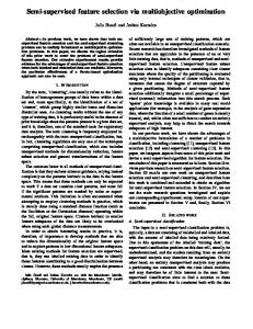
Let us perform the validation steps of the procedure, following their brief description given in the paper referred to in the Abstract. We shall confine ourselves to describing the first of them for the leukemia data only (for a similar analysis regarding the imputed lymphoma data, based on cRIgk , see [Drami´ nski et al., 2004]). The first validation step consists of two experiments. In the first experiment, 15,000 subsets of genes, each with 2,000 randomly selected genes, were drawn from the set of all 7,129 genes. For each such subset of features we thus have 38 samples from two classes, AML and AL. Each such set of 38 samples was randomly split 30 times into a training set of 24 and a test set of 14 samples. Finally, 450,000 trees were constructed on all the 450,000 training sets obtained, and their weighted accuracies were stored. The choice of the number of features for each sample was rather arbitrary, as the only requirement was to include sufficient randomness into the whole experiment. The second experiment was started with 50 random permutations of the class labels of the samples. Then, for each permutation, the experiment was run similarly to the former one. The only difference was that only 300 subsets ⋆ ⋆⋆

these authors contributed equally to whom correspondence should be addressed

2

Michal Drami´ nski et al.

Histogram - wAc curacy for or igin al class es 18 16 14 12 10 8 No of obs

6 4 2 0 0.685

0.686

0.687

0.688

0.689

0.690

0.691

0.692

0.693

0.694

0.695

w Accuracy

Fig. 1. wAcc for true classes: leukemia data

Histogram - w Accuracy for permuted classes 12

10

8

6 No of obs

4

2

0 0.28

0.29

0.30

0.31

0.32

0.33

0.34

0.35

0.36

0.37

0.38

0.39

0.40

0.41

w Accuracy

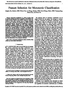
Fig. 2. wAcc for permuted classes: leukemia data

of 2,000 genes were randomly selected (that number of subsets multiplied by the number of permutations results in the same overall number, i.e. 15,000 of sets of samples, each with 2,000 features.).Hence, 450,000 trees were constructed and their wAcc’s stored. Results of both experiments are summarized by histograms in Fig’s. 1, 2, 3. It follows from them that the leukemia data can be considered informative. The second validation step begins with splitting the set of all d genes, ranked according to RIgk in the main step of the procedure, into two subsets: that of the 2b relatively most important genes and that of the remaining d − 2b genes. We set b = 100 for the leukemia data and b = 45 for the imputed lymphoma data. The second validation step consists again of two experiments. In the first experiment, b genes are randomly drawn 3,000 times from the set of the 2b relatively most important ones. Thus, for each such set of the b

Monte Carlo feature selection for supervised classification

3

Histogr am - w Accuracy 60%

50%

40%

30%

Percent of obs

20%

10%

0% 0.0

0.1

0.2

0.3

0.4

0.5

0.6

0.7

0.8

0.9

1.0

on the left for permuted class, on the right for original data

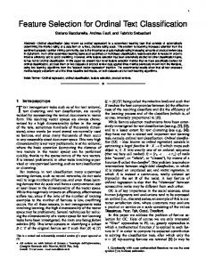
Fig. 3. wAcc for true and permuted classes: leukemia data Box Plot (golub200_200_pelne.sta 10v*60000c) 1.2

1.0

wAcc

0.8

0.6

0.4

0.2

0.0 100 out of top 200 100 out of 6929

Median 25%-75% Non-Outlier Range Outliers

experiment

Fig. 4. wAcc for 100-feature samples: leukemia data

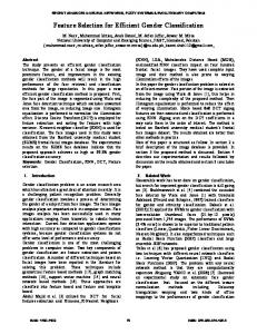
genes, one obtains a set of n samples, each sample with just b features. Now, each such set of samples is split 10 times at random into a training and a test set (as usual, each time 66% of samples are drawn at random for training in such a way as to preserve proportions of the classes from the complete set of training data). The 30,000 weighted accuracies thus obtained are stored. The second experiment is performed in the same way, except that each of the 3,000 sets of b genes is drawn from the set of the remaining d − 2b genes. The boxplots for wAcc, which resulted from our experiments, are given in Fig. 4 and Fig. 5. In this way, and for the leukemia and imputed lymphoma data, the claim that most important genes have been found by the main step of the procedure has been confirmed. For reasons explained at the end of Section 2.2 of the paper referred to in the Abstract, we suggest performing an additional confirmatory step, also outlined there (see the diagram in Fig. 6). For the leukemia data, 20 ALL

4

Michal Drami´ nski et al. Box Plot (alizadeh90_90.sta 4v*60000c) 1.1 1.0 0.9 0.8

wAcc

0.7 0.6 0.5 0.4 0.3 Median 25%-75% Non-Outlier Range Outliers

0.2 0.1 45 out of top 90

45 out of

45 out of 3936

Fig. 5. wAcc for 45-feature samples: lymphoma data

Experiment Final validation set

MCFS

2b highest ranking features

Data set Final testing set

Experiment 1 Final validation set

Draw b features fixed number of times

training Final testing set

wAcc testing

Experiment 2 Draw b features fixed number of times

Final validation set

training Final testing set

wAcc testing

Fig. 6. Block diagram for the confirmatory step; MCFS (Monte Carlo Feature Selection) is an acronym for the main step of the procedure

samples and 8 AML samples were drawn at random to the final validation set. For the lymphoma data, the final validation set comprised 26 DLCL samples, 7 FL samples and 9 CLL samples. In the former case, for the main step of the procedure we set m = 200, s = 10, 000 and t = 10. In the latter, we chose m = 100,s = 70, 000 and t = 20. In the second validation step, we used, respectively, b = 100 and b = 45 (as already earlier), and, respectively again, 10,000 and 100,000 sets of b genes were drawn in both experiments. The results obtained for the final test sets, not used in the main step in any way, are summarized by means of boxplots in Fig.’s 7 and 8. Thus, the earlier obtained rankings that were based on all samples may safely be claimed significant.

Monte Carlo feature selection for supervised classification

5

Box Plot (_acc_wAcc200_200.sta 3v*20000c) 1.1 1.0 0.9 0.8

wAcc

0.7 0.6 0.5 0.4 0.3 0.2

Median 25%-75% Non-Outlier Range Outliers

0.1 100 out of 200 100 out of 6930

Fig. 7. Confirmatory step: leukemia data (in the left boxplot, upper inner hinge coincides with the median) Box Plot (_acc_w Acc90_90 3v*200000c) 1.1 1.0 0.9 0.8

wAcc

0.7 0.6 0.5 0.4 0.3 Median 25%-75% Non-Outlier Range Outliers

0.2 0.1 45 out of 3936

45 out of 90

Fig. 8. Confirmatory step: lymphoma data

2

Monte Carlo Feature Selection (MCFS) algorithm with a rule based classifier

The original MCFS algorithm relies on using a decision tree classifier. In this section, we study the MCFS algorithm with rule-based, the so-called ADX, classifier in lien of the decision tree. ADX classifier has been proposed and implemented by Michal Drami´ nski [Drami´ nski, 2004]. 2.1

Definitions

Let D denote a database. Each row in a database is an event e (sometimes called an object), what means that D is a set of events/objects. Let |D| denote the number of events in D. Each column in database D corresponds to

6

Michal Drami´ nski et al.

one attribute of events. Attribute can be nominal such as color (e.g., possible values of color are: blue, red, green, etc.) or ordered such as height represented by an ordered set of values/levels (e.g., small, medium and high), or numerical such as height or weight measured, respectively, in inches and pounds. Attributes describe events in D. All possible combinations of values of attributes describing an event form a domain. We assume that D includes a special attribute called decision attribute d which determines class of each event. Thus, class is a value of d and each event in D has a defined class. We assume that the decision attribute has nominal values. Selector s is an expression that describes set of events using definition of one attribute. For example: color=blue; or weight>80. Each simple selector consists of a name of attribute, its value and an operator relating the two. More advanced/complex selector can include a list of nominal or ordered values (e.g. color=[blue, red]) or a range of numeric values (e.g. weight=(70;80] ). Both mentioned cases can be written as a set of simple selectors suitably combined into one advanced selector: ”color=[blue, red]” is the same as ”color=blue or color=red”, ”weight=(70;80]” is equivalent to ”weight>70 and weight≤80”. Selector s without any condition imposed on the attribute is called general and this kind of s will be presented as ”attribute=*” (e.g. color=* means any color). Let complex c denote a set of selectors and let length n of the complex denote the number of simple or advanced selectors contained in the complex. For example complex c = hs1 , s2 , s3 i has length 3. Complex is understood as a conjunction of selectors. Coverage cov of selector s is the number of events which satisfy condition in s (and are called covered events) divided by |D|. Coverage of any general selector is equal to 1.0. Coverage of c is the number of covered events (events which satisfy complex c, i.e., condition in s1 and in s2 and in s3 and so on) divided by |D|. Positive set Dp for a given class is the set of events whose decision attribute has the value corresponding to this class. During creation of rules for given value v of decision attribute d, all events that have v for d are called positive. All other events are called negative Dn . For a given class, positive coverage pcov of a given complex is the coverage on the subset of events which have the considered class. Negative coverage ncov of the complex is the coverage on the subset of events whose class is different from the considered class. By definition, strong rules determine classes, and hence their negative coverage is equal to 0. A complex which describes just one class can be called a strong rule (for that class). It means that if such a complex has ncov equal to 0 it implies only one class of events. We can say that probability of this class for such a rule is 1. If complex has ncov > 0 and pcov > ncov for a given class (value v of decision attribute d) it still describes this class but with some probability lesser then 1. This probability is usually called confidence or consistency of a rule. For strong rule confidence always equals 1. Set of complexes (disjunction of them) that describe one class we

Monte Carlo feature selection for supervised classification

7

call a ruleset. Set of rulesets that completely describe all classes (all values of decision attribute) we call a ruleset family.

2.2

The ADX algorithm — creation of a ruleset for one class

The general idea of ADX algorithm is based on the assumption that conjunction of selectors cannot have a bigger cov than minimal cov for each of these selectors. The main goal of the algorithm is to find the best ruleset (set of complexes such that each of them has possibly large pcov and possibly small ncov for each of the classes). If such rulesets exist, classification can be realized by measuring similarity of new unlabeled event to each ruleset (set of complexes for each class). Class which is most similar to the considered event will be chosen as a classifier decision. We assume that world is not perfect and probably input data either. It means that we can have in the data: ambiguities, noise, and unknown values.

Finding selectors base For a given class, for each value of each attribute in D, the algorithm finds pcov and ncov. It means that in the first step, the algorithm builds a set of contingency tables from a1 to am (where m denotes the number of all attributes with decision attribute d excluded). At this moment a new parameter can be defined. With this parameter, to be called minSelectorP osCoverage minimal acceptable positive coverage for a selector is determined. All selectors with smaller positive coverage than this parameter are deleted. All selectors that satisfy the condition determined by minSelectorP osCoverage are the basis for the next steps. Notice that in this step only simple selectors are selected. Size of selector base (number of selectors that satisfy minSelectorP osCoverage) affects complexity of later calculations.

Creation of candidates Complexes whose quality has not been evaluated yet are called candidates. Creation of such complexes with length 2 is very simple. These are all possible selectors’ pairs excluding pairs where both selectors are based on the same attribute. Notice that complex (of length 2) c1 = hs1 , s2 i equals c2 = hs2 , s1 i, because each complex consists of conjunction of selectors. There is an important issue about creation of complexes longer than 2. To create a new complex candidate, the algorithm uses two complexes with length smaller by 1, which can be called parents. Parent complexes need to have common part of length n − 1 (where n denotes the length of parents complexes). For example complex c1 = hs1 , s2 , s3 i and c2 = hs2 , s3 , s5 i can be used to create c3 = hs1 , s2 , s3 , s5 i. Creation of complexes with length 2 is based on simple selectors. Complexes with length 3 are based on complexes with length 2 and so on.

8

Michal Drami´ nski et al.

Estimation of candidates’ quality After creation of each candidates set there is a need to separately estimate quality of each newly created complex. During the estimation process, for each complex candidate there is calculated positive and negative coverage (pcov and ncov) on a training set. This can be done by calculation of how many positive and negative events are covered by the complex considered. The best complexes become parents and are used to create in the next iteration complex candidates 1 selector longer. Some quality measure Q is used to compare complexes and it is defined as follows Q = (pcov−ncov)(1−ncov)u , where u equals to 1 for estimation of candidates’ process and u = 1/2 for later final selection. Complexes that do not cover any positive event (pcov = 0) are useless and are deleted. Selection of parents Selection is a process during which ADX selects complexes (using estimation measures pcov and ncov) as parents from which next candidates are created. The set of selected complexes will be used in the next iteration as a parent set. However, parameter searchBeam is used to limit the number of complexes to be a parent in the next step. This parameter uses measures Q to select candidates for the next step. After the evaluation process, selection of a set of best complexes is performed that can be used to create next complexes of length greater by 1. Complexes which were not selected to be parents are stored for final selection. Parameter searchBeam controls the scope of exploration but also affects learning time. With increasing searchBeam exploration grows also but, unfortunately, learning time grows too. Once the set of parents is selected new candidates can be created (complexes that are 1 selector longer). The algorithm can be stopped when the set of new candidates is empty (if there are no parents that have common part of n − 1 length). Merging of complexes and final selection of ruleset After creation of all possible complexes, the algorithm decreases the number of them and improves their quality. If complexes are based on the same attribute set and only one selector has different value then it is possible to merge such complexes. Instead of old complexes the new one is added. For example: hA = 1, B = 3, C = 4i⊕hA = 1, B = 3, C = 7i =⇒ hA = 1, B = 3, C = [4, 7]i, where new selector is C = [4, 7]. For the resulting complex pcov and ncov are the sums of corresponding coverages of deleted complexes. The main criterion that allows for merging of two complexes is the increase of Q for the outcome complex compared to any component complexes. In final selection step - from the whole set of stored rules we have to select the most appropriate set that can be used for later prediction. Selection of final rules is based on measure Q and selecting fixed number of rules f inalBeam. First of all, complexes are sorted by Q and starting from the highest Q, they are added one by one to the final set. After adding a complex it is

Monte Carlo feature selection for supervised classification

9

retained in the set, √ if its inclusion does not decrease the value of Qr . Measure Qr = (S p − S n ) 1 − S n is very similar to Qu=1/2 where S p and S n are sums of suitable factors over all rules in the final ruleset. The factors S p and S n are sums of scores (to be described in the next section) obtained on random subset of training events – S p is a sum for positive events e and S n for negative ones. X Sp = S(e) (1) e∈D p

Sn =

X

S(e)

(2)

e∈D n

The idea is to select complexes that maximize score for positive events and minimize it for the negative set – both for randomly selected subset of training events. 2.3

Classification in ADX

For prediction, the ADX algorithm uses the set of final rules, obtained from final selection. For each of the rulesets, subset of rules that cover an event are selected and the score measure is calculated for each such subset. The highest score determines the class label. The score measure combines pcov, ncov and prob of rules that cover the event, where prob denotes probability of positive class occurrence for a given rule. The score measure can be defined in any of the following ways: 1.

p−n |r| P −N |R|

S0 = 2.

(3)

S1 =

p−n P −N

(4)

S2 =

p N ∗ P n

(5)

n p ∗ [1 − ] P N

(6)

Y (1 − prob(r))

(7)

P

(8)

3.

4. S3 = 5. S4 = 1 − 6. S5 =

r

r

prob(r) r

10

Michal Drami´ nski et al.

7. S6 =



S5

S7 =



S4

P p

if

V

S5c = 1

if

V

S4c = 1

8. P p

where:

c

c

• • • • • •

p – denotes sum pcov of rules that cover tested event n – denotes sum ncov of rules that cover tested event P – denotes sum pcov of rules for a given class N – denotes sum ncov of rules for a given class r – denotes subset of rules that cover an event prob – probability of occurrence of positive class if the rule covers the event • c – is a class label

The experiments have proven that the most universal measure is S6 and gives very good and stable classification results. 2.4

Integration of ADX into MCFS

The original version of MCFS is based on decision tree classifier but if any other classifier meets two simple criteria there is no problem to integrate it: • It works at least as fast as a decision tree - because we would like to train/test thousands of classifiers in reasonable time. • It is possible to propose RIgk measure for such classifier. Experiment show that the first criterion is definitely fulfilled by ADX classifier. To fulfill the second criterion the following measure RIgk has to be introduced: RIgk =

st X

σ=1

(wAcc)u

X

v

Q(rgk (σ)) (cov(rgk (σ))) ,

(9)

rgk (σ)

The proposed measure is similar to RI for the decision tree classifier. In the above formula rgk (σ) denotes the rule that contains selector based on gk (rule plays the same role as nodes in RI). Instead of Information Gain for a tree node we can now use Q of the rule. Coverage of the rule plays the role of the fraction of events tested in a particular node of the decision tree. Note that from ADX we can obtain separate sets of rules, each of them pertaining to a different class. Therefore it is possible to construct separate rankings of genes for different classes.

Monte Carlo feature selection for supervised classification

2.5

11

Top ranking genes by two implementations of the MCFS algorithm

It is interesting to see if the rankings of genes provided by two different implementations of the MCFS algorithm, one with decision trees and another with ADX rule based classifiers, can be considered overlapping to a sufficiently large extent. For our two example data sets (Alizadeh and Golub), we have found that the groups (of whatever but equal size, from tens to hundreds) of top ranking genes obtained by the two procedures, overlap in about 50% for the Alizadeh et al. and about 75% for the Golub et al. data. This result is illustrated in tables 1 and 2 for the sets of 45 and 90 top ranking features. Given that the ranking is made between thousands of genes, the overlap can be considered reasonably high.

algorithm

J48

ADX

J48

x

21

ADX

41

x

Table 1. Overlap of top rankings obtained from c4.5 and ADX (top right 45 top features, bottom left 90 top features) – Alizadeh et al. data

algorithm

J48

ADX

J48

x

33

ADX

65

x

Table 2. Overlap of top rankings obtained from c4.5 and ADX (top right 45 top features, bottom left 90 top features) – Golub et al. data

References ´ [Drami´ nski et al., 2004] Drami´ nski, M., Koronacki, J., Cwik, J. and Komorowski, J. (2004) Monte Carlo Gene Screening for Supervised Classification. In: Current Issues in Data and Knowledge Engineering, B. De Baets, R. de Caluwe, G. de Tr, J. Fodor, J. Kacprzyk, S. Zadrozny (eds.), Exit, Warsaw. [Drami´ nski, 2004] Drami´ nski M. (2004) ADX Algorithm: A brief Description of a Rule Based Classifier. Proceedings of the New Trends in Intelligent Information Processing and WebMining IIS’2004 Symposium, Zakopane, Poland, SpringerVerlag.

12

A

Michal Drami´ nski et al.

Top ranging genes for leukemia data MCFS+J48

Ranging of the top 200 highly estimated genes obtained of MCFS using decision tree (leukemia data): 1. 2. 3. 4. 5. 6. 7. 8. 9. 10. 11. 12. 13. 14. 15. 16. 17. 18. 19. 20. 21. 22. 23. 24. 25. 26. 27. 28. 29. 30. 31. 32. 33. 34. 35. 36. 37. 38. 39. 40.

X95735 at M31166 at M27891 at M55150 at D88422 at M23197 at M98399 s at U50136 rna1 at M21551 rna1 at M27783 s at M54995 at U02020 at M77142 at M81933 at X70297 at Y12670 at U46499 at M83652 s at U46751 at L09209 s at M16038 at D14874 at M84526 at M92287 at M31523 at X62654 rna1 at M31303 rna1 at D49950 at U22376 cds2 s at J05243 at D26308 at X90858 at J04615 at X74262 at L08177 at U37055 rna1 s at X87613 at M80254 at X62320 at J04990 at

Monte Carlo feature selection for supervised classification

41. 42. 43. 44. 45. 46. 47. 48. 49. 50. 51. 52. 53. 54. 55. 56. 57. 58. 59. 60. 61. 62. 63. 64. 65. 66. 67. 68. 69. 70. 71. 72. 73. 74. 75. 76. 77. 78. 79. 80. 81. 82. 83. 84. 85.

L47738 at M29540 at M91432 at U85767 at M24400 at M96326 rna1 at L05148 at M11722 at U12471 cds1 at U82759 at X59417 at X04085 rna1 at HG4321-HT4591 at U16954 at M22324 at U41813 at HG2981-HT3127 s at X14008 rna1 f at M12959 s at M62762 at X06182 s at M81695 s at M63138 at D87076 at M28130 rna1 s at D14664 at X17042 at D38073 at M57731 s at AFFX-HUMTFRR/M11507 3 at U09087 s at HG627-HT5097 s at D87742 at X85116 rna1 s at Y00787 s at M69043 at L08246 at M58297 at D26156 s at HG1612-HT1612 at L09717 at M22960 at M13452 s at X07743 at U62136 at

13

14

86. 87. 88. 89. 90. 91. 92. 93. 94. 95. 96. 97. 98. 99. 100. 101. 102. 103. 104. 105. 106. 107. 108. 109. 110. 111. 112. 113. 114. 115. 116. 117. 118. 119. 120. 121. 122. 123. 124. 125. 126. 127. 128. 129. 130.

Michal Drami´ nski et al.

X15949 at AF009426 at D10495 at M25897 at Z48501 s at M31158 at J03589 at X51521 at U38846 at X16546 at M31211 s at U73737 at M86406 at X58431 rna2 s at X62535 at HG2855-HT2995 at M83667 rna1 s at M63379 at U97105 at X74801 at L34600 at HG2379-HT3996 s at J04621 at AF012024 s at D38128 at U67963 at U79734 at M95678 at Z69881 at U41767 s at M29194 at Z49194 at L42572 at L38608 at M20203 s at J03930 at U72621 at X52142 at U32944 at J03801 f at M28209 at U20998 at M19507 at U90902 at D38522 at

Monte Carlo feature selection for supervised classification

131. 132. 133. 134. 135. 136. 137. 138. 139. 140. 141. 142. 143. 144. 145. 146. 147. 148. 149. 150. 151. 152. 153. 154. 155. 156. 157. 158. 159. 160. 161. 162. 163. 164. 165. 166. 167. 168. 169. 170. 171. 172. 173. 174. 175.

L20941 at L19779 at M95178 at X52056 at M83221 at M13792 at X77533 at HG4582-HT4987 at M26708 s at M28170 at L25931 s at HG2788-HT2896 at L41870 at U43292 at X61587 at U00802 s at U88629 at S82470 at L13278 at S82185 at U53225 at M80899 at U19878 at X66533 at HG4755-HT5203 s at M25809 at L11669 at U40369 rna1 at HG3494-HT3688 at M68891 at X64364 at U72936 s at M29696 at M75715 s at L28821 at AFFX-HUMTFRR/M11507 M at M93056 at U29175 at X16901 at X80907 at X17094 at M61853 at HG3454-HT3647 at X66401 cds1 at U61836 at

15

16

176. 177. 178. 179. 180. 181. 182. 183. 184. 185. 186. 187. 188. 189. 190. 191. 192. 193. 194. 195. 196. 197. 198. 199. 200.

B

Michal Drami´ nski et al.

M32304 s at X63753 at X83490 s at Z15115 at U90552 s at X57579 s at Z32765 at M86873 s at M29971 at L13329 at D31887 at U58034 at D88378 at U31342 at L20321 at Z18948 at M20642 s at L49219 f at U77396 at M19045 f at D86967 at AF005043 at D82346 at Y00339 s at J04027 at

Top ranging genes for lymphoma data MCFS+J48

Ranging of the top 200 highly estimated genes obtained of MCFS using decision tree (lymphoma data - not imputed data): 1. 2. 3. 4. 5. 6. 7. 8. 9. 10. 11. 12. 13. 14.

GENE1622X GENE1602X GENE1613X GENE1553X GENE530X GENE1610X GENE1647X GENE653X GENE1606X GENE2426X GENE622X GENE2402X GENE1661X GENE598X

Monte Carlo feature selection for supervised classification

15. 16. 17. 18. 19. 20. 21. 22. 23. 24. 25. 26. 27. 28. 29. 30. 31. 32. 33. 34. 35. 36. 37. 38. 39. 40. 41. 42. 43. 44. 45. 46. 47. 48. 49. 50. 51. 52. 53. 54. 55. 56. 57. 58. 59.

GENE2668X GENE669X GENE588X GENE537X GENE639X GENE2553X GENE542X GENE1673X GENE685X GENE454X GENE844X GENE640X GENE2368X GENE1607X GENE1635X GENE1605X GENE2404X GENE1632X GENE584X GENE834X GENE1603X GENE1648X GENE849X GENE642X GENE1662X GENE524X GENE694X GENE617X GENE771X GENE1672X GENE1611X GENE651X GENE620X GENE464X GENE2589X GENE626X GENE689X GENE1637X GENE646X GENE563X GENE2356X GENE586X GENE2373X GENE2097X GENE2391X

17

18

60. 61. 62. 63. 64. 65. 66. 67. 68. 69. 70. 71. 72. 73. 74. 75. 76. 77. 78. 79. 80. 81. 82. 83. 84. 85. 86. 87. 88. 89. 90. 91. 92. 93. 94. 95. 96. 97. 98. 99. 100. 101. 102. 103. 104.

Michal Drami´ nski et al.

GENE760X GENE1644X GENE1599X GENE2360X GENE3497X GENE2340X GENE2547X GENE236X GENE447X GENE712X GENE650X GENE717X GENE1625X GENE616X GENE2240X GENE2554X GENE2190X GENE2345X GENE1617X GENE631X GENE816X GENE636X GENE2324X GENE625X GENE802X GENE2244X GENE1537X GENE459X GENE2270X GENE655X GENE977X GENE1192X GENE641X GENE3621X GENE1619X GENE728X GENE1676X GENE2357X GENE2346X GENE632X GENE729X GENE1623X GENE2374X GENE649X GENE538X

Monte Carlo feature selection for supervised classification

105. 106. 107. 108. 109. 110. 111. 112. 113. 114. 115. 116. 117. 118. 119. 120. 121. 122. 123. 124. 125. 126. 127. 128. 129. 130. 131. 132. 133. 134. 135. 136. 137. 138. 139. 140. 141. 142. 143. 144. 145. 146. 147. 148. 149.

GENE2364X GENE675X GENE659X GENE647X GENE528X GENE1731X GENE611X GENE3792X GENE812X GENE1612X GENE1975X GENE638X GENE2109X GENE508X GENE2271X GENE765X GENE770X GENE1507X GENE768X GENE1747X GENE788X GENE734X GENE292X GENE2096X GENE738X GENE1615X GENE2253X GENE1583X GENE633X GENE735X GENE663X GENE2110X GENE531X GENE455X GENE3704X GENE2370X GENE2310X GENE1295X GENE546X GENE2378X GENE2403X GENE709X GENE1656X GENE838X GENE733X

19

20

150. 151. 152. 153. 154. 155. 156. 157. 158. 159. 160. 161. 162. 163. 164. 165. 166. 167. 168. 169. 170. 171. 172. 173. 174. 175. 176. 177. 178. 179. 180. 181. 182. 183. 184. 185. 186. 187. 188. 189. 190. 191. 192. 193. 194.

Michal Drami´ nski et al.

GENE2113X GENE681X GENE473X GENE1204X GENE2166X GENE786X GENE1220X GENE457X GENE1616X GENE539X GENE2221X GENE3770X GENE2293X GENE710X GENE541X GENE2076X GENE742X GENE2108X GENE682X GENE740X GENE2321X GENE2251X GENE1631X GENE3880X GENE543X GENE303X GENE593X GENE691X GENE714X GENE1600X GENE2214X GENE2328X GENE1674X GENE648X GENE1732X GENE3635X GENE307X GENE3384X GENE713X GENE1636X GENE2339X GENE3787X GENE2429X GENE703X GENE884X

Monte Carlo feature selection for supervised classification

195. 196. 197. 198. 199. 200.

C

21

GENE3786X GENE1748X GENE529X GENE676X GENE2548X GENE2424X

Top ranging genes for leukemia data MCFS+ADX

Ranging of the top 200 highly estimated genes obtained of MCFS using rule based classifier (leukemia data): 1. 2. 3. 4. 5. 6. 7. 8. 9. 10. 11. 12. 13. 14. 15. 16. 17. 18. 19. 20. 21. 22. 23. 24. 25. 26. 27. 28. 29. 30. 31. 32. 33.

X95735 at M55150 at M31166 at M27891 at M77142 at D88422 at X70297 at U46499 at U50136 rna1 at M27783 s at M91432 at L09209 s at M23197 at M16038 at Y12670 at D14874 at U22376 cds2 s at M92287 at X62654 rna1 at U02020 at X74262 at M81933 at M31523 at U41813 at M12959 s at M28130 rna1 s at U85767 at J03930 at M84526 at U62136 at X59417 at X90858 at U12471 cds1 at

22

34. 35. 36. 37. 38. 39. 40. 41. 42. 43. 44. 45. 46. 47. 48. 49. 50. 51. 52. 53. 54. 55. 56. 57. 58. 59. 60. 61. 62. 63. 64. 65. 66. 67. 68. 69. 70. 71. 72. 73. 74. 75. 76. 77. 78.

Michal Drami´ nski et al.

X04085 rna1 at U46751 at U09087 s at J04615 at M83652 s at U73737 at L47738 at X80907 at X74801 at X07743 at M54995 at J05243 at L27584 s at Y00787 s at U32944 at M21551 rna1 at M63138 at D38073 at M31303 rna1 at M11722 at AF009426 at D10495 at U38846 at L42572 at AFFX-HUMTFRR/M11507 3 at M31158 at X52142 at Z69881 at X15949 at HG4321-HT4591 at D26156 s at M28170 at X85116 rna1 s at L41870 at X06182 s at D38522 at M31211 s at X62320 at U29175 at M29540 at Y11710 rna1 at D26308 at M63488 at M96326 rna1 at X58431 rna2 s at

Monte Carlo feature selection for supervised classification

79. 80. 81. 82. 83. 84. 85. 86. 87. 88. 89. 90. 91. 92. 93. 94. 95. 96. 97. 98. 99. 100. 101. 102. 103. 104. 105. 106. 107. 108. 109. 110. 111. 112. 113. 114. 115. 116. 117. 118. 119. 120. 121. 122. 123.

X61587 at U65928 at M80254 at U26266 s at HG2810-HT2921 at Z49194 at HG1612-HT1612 at Z15115 at M58297 at X57579 s at D86479 at X66533 at J03801 f at L28821 at X62535 at M98399 s at S50223 at S82185 at U41767 s at D63880 at J03589 at X66401 cds1 at L08246 at X77533 at AF012024 s at U72936 s at U31342 at M19045 f at U02493 at X14008 rna1 f at M54915 s at HG2855-HT2995 at U72621 at M94633 at U35451 at L38608 at M55040 at M23178 s at M29696 at U90546 at U82759 at U73960 at L07648 at M24349 s at M22960 at

23

24

124. 125. 126. 127. 128. 129. 130. 131. 132. 133. 134. 135. 136. 137. 138. 139. 140. 141. 142. 143. 144. 145. 146. 147. 148. 149. 150. 151. 152. 153. 154. 155. 156. 157. 158. 159. 160. 161. 162. 163. 164. 165. 166. 167. 168.

Michal Drami´ nski et al.

M62762 at X59350 at L13278 at D82346 at U20998 at U84487 at U05259 rna1 at D14664 at S79854 at X17042 at M83667 rna1 s at M24400 at D49950 at U27460 at U16307 at M25897 at X98261 at U59321 at U26173 s at X76648 at D88270 at U67963 at M81695 s at U79274 at D38128 at M74088 s at D43950 at Y13896 at M29194 at U66838 at U28413 at X63469 at U31556 at AC002115 cds4 at M22324 at M95678 at D86983 at X16546 at U47928 at M63379 at S82470 at J04990 at HG2788-HT2896 at D43682 s at M15059 at

Monte Carlo feature selection for supervised classification

169. 170. 171. 172. 173. 174. 175. 176. 177. 178. 179. 180. 181. 182. 183. 184. 185. 186. 187. 188. 189. 190. 191. 192. 193. 194. 195. 196. 197. 198. 199. 200.

D

25

X87613 at U90902 at X64072 s at U90552 at M69043 at X54326 at M86406 at Z19002 at X66899 at Z68747 at X97748 s at M63438 s at L25931 s at U28833 at U94836 at M37435 at U28758 s at L10386 at D87742 at HG4332-HT4602 at U00802 s at M19507 at X83490 s at HG4316-HT4586 at M65214 s at D80001 at D83785 at X63753 at U49020 cds2 s at U50733 at M60527 at M13792 at

Top ranging genes for lymphoma data MCFS+ADX

Ranging of the top 200 highly estimated genes obtained of MCFS using rule based classifier (lymphoma data): 1. 2. 3. 4. 5. 6. 7.

GENE1622X GENE1618X GENE1617X GENE1602X GENE659X GENE1744X GENE1619X

26

8. 9. 10. 11. 12. 13. 14. 15. 16. 17. 18. 19. 20. 21. 22. 23. 24. 25. 26. 27. 28. 29. 30. 31. 32. 33. 34. 35. 36. 37. 38. 39. 40. 41. 42. 43. 44. 45. 46. 47. 48. 49. 50. 51. 52.

Michal Drami´ nski et al.

GENE1637X GENE1636X GENE1616X GENE1644X GENE1702X GENE1662X GENE1647X GENE1661X GENE653X GENE766X GENE1610X GENE622X GENE530X GENE1553X GENE1632X GENE735X GENE1613X GENE1634X GENE1648X GENE1635X GENE712X GENE1643X GENE834X GENE1645X GENE1607X GENE1641X GENE1625X GENE1649X GENE1640X GENE1627X GENE588X GENE2368X GENE1663X GENE2402X GENE675X GENE598X GENE1603X GENE633X GENE710X GENE669X GENE620X GENE625X GENE1633X GENE1753X GENE1731X

Monte Carlo feature selection for supervised classification

53. 54. 55. 56. 57. 58. 59. 60. 61. 62. 63. 64. 65. 66. 67. 68. 69. 70. 71. 72. 73. 74. 75. 76. 77. 78. 79. 80. 81. 82. 83. 84. 85. 86. 87. 88. 89. 90. 91. 92. 93. 94. 95. 96. 97.

GENE1595X GENE1609X GENE689X GENE1608X GENE721X GENE586X GENE641X GENE1646X GENE1650X GENE1660X GENE1639X GENE651X GENE642X GENE1638X GENE616X GENE1606X GENE639X GENE1693X GENE1674X GENE399X GENE631X GENE491X GENE1599X GENE1596X GENE1692X GENE473X GENE655X GENE2110X GENE647X GENE626X GENE1204X GENE1631X GENE648X GENE1651X GENE738X GENE844X GENE1295X GENE531X GENE1652X GENE636X GENE589X GENE1698X GENE711X GENE1730X GENE1549X

27

28

98. 99. 100. 101. 102. 103. 104. 105. 106. 107. 108. 109. 110. 111. 112. 113. 114. 115. 116. 117. 118. 119. 120. 121. 122. 123. 124. 125. 126. 127. 128. 129. 130. 131. 132. 133. 134. 135. 136. 137. 138. 139. 140. 141. 142.

Michal Drami´ nski et al.

GENE611X GENE1696X GENE1671X GENE2395X GENE1623X GENE765X GENE1653X GENE698X GENE1514X GENE2403X GENE1629X GENE558X GENE1537X GENE716X GENE1539X GENE555X GENE652X GENE896X GENE2404X GENE537X GENE524X GENE2426X GENE717X GENE650X GENE638X GENE685X GENE2555X GENE1615X GENE2391X GENE977X GENE236X GENE1656X GENE2668X GENE682X GENE542X GENE719X GENE508X GENE709X GENE2244X GENE646X GENE727X GENE1545X GENE1516X GENE1624X GENE527X

Monte Carlo feature selection for supervised classification

143. 144. 145. 146. 147. 148. 149. 150. 151. 152. 153. 154. 155. 156. 157. 158. 159. 160. 161. 162. 163. 164. 165. 166. 167. 168. 169. 170. 171. 172. 173. 174. 175. 176. 177. 178. 179. 180. 181. 182. 183. 184. 185. 186. 187.

GENE2339X GENE697X GENE1684X GENE649X GENE660X GENE2554X GENE676X GENE534X GENE1612X GENE595X GENE1614X GENE2400X GENE1223X GENE635X GENE1697X GENE2354X GENE563X GENE1578X GENE446X GENE1600X GENE1655X GENE654X GENE681X GENE587X GENE1523X GENE775X GENE585X GENE2190X GENE1736X GENE1673X GENE725X GENE506X GENE2373X GENE2345X GENE1679X GENE771X GENE2346X GENE657X GENE783X GENE1605X GENE565X GENE734X GENE645X GENE868X GENE1581X

29

30

188. 189. 190. 191. 192. 193. 194. 195. 196. 197. 198. 199. 200.

Michal Drami´ nski et al.

GENE694X GENE619X GENE695X GENE568X GENE538X GENE490X GENE2392X GENE464X GENE786X GENE529X GENE1654X GENE520X GENE632X