MOPSO-based predictive control strategy for efficient ... - DergiPark

Turkish Journal of Electrical Engineering & Computer Sciences http://journals.tubitak.gov.tr/elektrik/

Turk J Elec Eng & Comp Sci (2017) 25: 2968 – 2985 ¨ ITAK ˙ c TUB ⃝ doi:10.3906/elk-1608-115

Research Article

MOPSO-based predictive control strategy for efficient operation of sensorless vector-controlled fuel cell electric vehicle induction motor drives 1

Adel Abdelaziz Abdelghany ELGAMMAL1,∗, Mohamed Fathy EL-NAGGAR2,3 Department of Energy, University of Trinidad and Tobago, Point Lisas Campus, Couva, Trinidad and Tobago 2 Department of Electrical Engineering, Prince Sattam bin Abdulaziz University, Al Kharj, Saudi Arabia 3 Department of Electrical Engineering, Helwan University, Helwan, Egypt

Received: 11.08.2016

•

Accepted/Published Online: 14.11.2016

•

Final Version: 30.07.2017

Abstract: This paper introduces an optimal control strategy of model-based predictive control (MPC) based on multiobjective particle swarm optimization (MOPSO) for a sensorless vector control induction motor, which is used in a fuel cell electric vehicle drive system. The proposed MPC-MOPSO algorithm is implemented to tune the weighting parameters of the MPC controller to tackle all the conflicting objective functions. The paper handles the following fitness functions: minimizing the speed error, minimizing the torque ripple, minimizing the DC-link voltage ripple, and minimizing machine flux ripple. Computer simulations studies have been completed utilizing MATLAB/Simulink with a specific end goal of assessing the dynamic performance of the proposed MPC-MOPSO optimal controller and comparing it with single-objective particle swarm optimization and traditional PI controllers. The simulation results demonstrate the good dynamic response of the proposed MPC-MOPSO optimal tuning strategy over the traditional PI controllers for more accurate tracking performance through the whole speed range, especially at starting conditions and load change disturbances. Key words: Electric vehicle, fuel cell, sensorless vector control, multiobjective particle swarm optimization, model-based predictive control

1. Introduction Concern about air contamination, global warming, and the quick consumption of fossil fuels such as oil, gas, and coal has prompted the proposition of fuel cell electric vehicles (FC-EVs) to replace traditional vehicles [1]. Usually, batteries are utilized for all types of EVs as a second rechargeable energy source to implement good acceleration and regenerative braking while the main energy source such as the FC is utilized to give extended driving range [2]. In spite of the fact that FCs show great power ability in steady-state operation, the technical restrictions of FCs such as low productivity in a low load request, moderate power transfer rate in transient operation, and high cost for each watt make the reaction of the FC in transient and momentary crest power requests generally poor. In this way, batteries and/or superconductors are utilized with the FC. However, the batteries introduce a few downsides, such as short lifecycle, long charging time, and low power densities, despite giving noteworthy high-energy density potential, and they might be enormously influenced by high current discharges [3]. The induction motors that are used in the EVs could be controlled by field-oriented control (FOC) to operate at their optimum efficiency, torque, and speed. In the last few years, FOC drives have ∗ Correspondence:

2968

[email protected]

ELGAMMAL and EL-NAGGAR/Turk J Elec Eng & Comp Sci

been widely utilized for induction motor optimal speed control [4]. Because of their simple control structure and inexpensive cost, PID and hysteresis current controllers are commonly used in traditional FOC to achieve smooth transient operation of the induction motor drive [5]. In any case, the PI controller demonstrates poor transient reaction against system parametric variety and sudden load change influence, particularly during lowspeed operations. The trend in industrial applications is to implement sensorless vector control techniques to estimate the motor speed and flux using computational methods instead of using speed sensors to strengthen the drive system reliability [6]. The generally utilized strategies for speed observation are the model reference adaptive system [7,8], neural networks [9], extended Kalman filter [10,11], and nonlinear observer [12]. A comprehensive literature review of optimal control of induction motor drives based on sensorless vector control was given in [13]; however, new solutions should be suggested to overcome a few issues connected with sensorless vector control [14]. Current research works focus on wide speed ranges, especially very low speed ranges [15], or inaccuracy and IM parameter variations [16]. Intelligent techniques such as neural networks, fuzzy control, and genetic algorithms have been utilized to handle the nonlinearities and uncertainties of the IM parameters [17–20]. Model-based predictive control (MPC) has become a major control technology due to its ability to deal with a dynamic optimization problem with physical constraints that come from the industrial applications and control process [21]. MPC relies on the dynamic models of the process to compute a vector of optimal control signals by solving an optimization problem online considering the process constraints to minimize the future signal error, which is the difference between the desired signal and the future outputs predicted by the process model. At that point, the first signal of the optimal input vector is connected to the plant and this strategy from the prediction and optimization with new optimal input is repeated in the following sampling interval [22]. Comparing the performance of MPC to conventional PID controllers, the main disadvantage of MPC is that it is a generally more perplexing controller and it requires more time for online prediction, particularly when constraints exist. However, the literature has shown that the performance usually indicates obvious MPC predominance [23]. MPC has been utilized in optimal speed/torque control for induction motor drive systems [24] and joined with speed/flux estimators [25]. Recently, FLC control and PSO approaches have been implemented in the automatic tuning of model predictive control parameters [26–28]. In this paper, the MPC-multiobjective particle swarm optimization (MOPSO) optimal control approach is implemented to control the speed, torque, flux, and DC voltage for a sensorless vector control IM drive, which is intended to be implemented in a FC-EV drive system. The proposed MPC-MOPSO algorithm is implemented to tune the weighting parameters of the MPC controller to handle the following fitness functions: minimizing the speed error, minimizing the torque ripple, minimizing the DC-link voltage ripple, and minimizing machine flux ripple while considering the provided drive system constraints. The control signal is predicted by MPC based on the current control variables, the actual signal error, and the predicted future output of the model. The dynamic performance of the MPC-MOPSO controller is tested with different speed tracks and load disturbance and compared using MATLAB/Simulink with the traditional PI controller and single-objective particle swarm optimization (SOPSO). SOPSO and MOPSO can be utilized to figure out this multiobjective optimization problem. In SOPSO, a single weighted objective function may be formed from all fitness functions to obtain a single solution, while MOPSO finds a set of acceptable trade-off optimal solutions, which is called the Pareto front. The main point of interest in MOPSO is that it does not need a priori knowledge about the relative significance of the targets [29–32]. This paper is organized as follows: Section 2 introduces the dynamic model of the induction motor. Section 3 outlines the fundamental structure of the model-based predictive control. Section 4 presents the system arrangement of a typical fuel cell/supercapacitor/battery EV. Section 5 demonstrates the proposed MOPSO and SOPSO optimal

2969

ELGAMMAL and EL-NAGGAR/Turk J Elec Eng & Comp Sci

algorithms. Section 6 shows the dynamic simulations using MATLAB/Simulink. Finally, particular important conclusions are presented in Section 7. 2. The sensorless control of the IM The dynamic state-space model of the IM can be represented using the d − q reference frame as follows [33]: 

ids

 i d   qs  dt  λdr λqr





−γ

    −ωs =   ηL m   0

ωs

ηµ

ωr µ

−γ

−ωr µ

ηµ

0

−η

ηLm

−ωsl

Te =



η=

Rr Lr ;

1 σLs

    0 +   0   0

   iqs   ωsl    λdr λqr −η

0 1 σLs

0 0



vds

   vqs   0  0

   ,  

3P Lm (iqs λdr − ids λqr ) , 4Lr

where: σ =1−





ids

L2m Ls Lr ;

µ=

γ=

Lm σLs Lr ;

1 σLs

( Rs +

L2m L2r Rr

(1)

(2) ) ; (3)

ωsl = ωs − ωr

vds and vqs are d − q stator voltage components, ids and iqs are d− q stator current components, λdr and λqr are d − q rotor flux linkage components, ωs is stator angular speed, ωr is mechanical rotor speed, ωsl is slip angular speed, Te is the electromagnetic torque, P is the number of pole pairs, Rs and Rr are stator and rotor resistance referred to the stator, and Ls , Lr , and Lm are stator, rotor, and mutual inductances referred to the stator. The speed can be evaluated by the model referencing adaptive system, which primarily comprises the reference and adaptive models. The adjustment strategy creates the assessed speed where the calculated values of the reference model are compared with the output of the adjustable model until the difference between the two models reaches zero. The reference model represents the stator voltage equation in the stator reference frame, which can be composed as: d dt

[

λsdr λsqr

]

Lr = Lm

[

s vds s vqs

]

Lr − Lm

[ ( ) d Rs + σLs dt 0

0 ( ) d Rs + σLs dt

][

isds isqs

] .

(4)

The adaptive model represents the rotor voltage equation of the IM in the stator reference frame, which can be written as: [ [ ] ] [ ][ ] s ˆs ωr − T1r −ˆ λ λsdr d Lm ids dr , (5) = + ˆs dt λ Tr ω ˆr − T1r isqs λsqr qr ˆ s and λ ˆ s are the estimated where Tr is the rotor circuit time constant, ω ˆ r is the adaptive rotor speed, and λ qr dr d − q rotor flux linkages in the stationary reference frame. The signal of the speed tuning error εcan be calculated as: ˆ s λs − λ ˆ s λs . ε=λ dr qr qr dr

(6)

With the correct estimated rotor speed, the two flux linkages calculated by the two models should coordinate. An adjustment calculation with the PI control can be utilized to tune the speed until the two flux values 2970

ELGAMMAL and EL-NAGGAR/Turk J Elec Eng & Comp Sci

coordinate:

( ) ) Ki ( ˆ s s ˆ s λs . ω ˆ r = Kp + λdr λqr − λ qr dr S

(7)

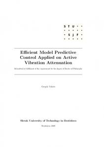
3. Model-based predictive control MPC is a type of control that utilizes the accurate model of the plant to predict the future performance of a process. The control action is obtained by solving a constrained optimization problem at every sample interval to minimize the difference between the estimated future outputs and the reference value through the use of minimum control energy and satisfying the constraints of the plant, as shown in Figure 1. There are mainly four available components:

Figure 1. General structure of model predictive controller.

1. The process model: for each instance k, the system model is utilized to predict the future response of the controlled plant (y (k), y (k + 1), y (k + 2), . . . , y (k + N P – 1)) over a specified prediction horizon N P . In MPC it is assumed that the model can be formed as a state-space model, as shown in the following equation: xk+1 = Axk + Buk yk = Cxk + Duk

.

(8)

1. The cost function: for each iteration k, the MPC controller calculates a sequence of future control actions (u (k), u (k + 1), u (k + 2),. . . , u (k + N c – 1)) over a specified control horizon N c such that the objective function is optimized (minimized or maximized) subject to the specified constraints. The objective function is generally a combination of weighted sum of square predicted errors and square future control values. 2. The optimizer to optimize the future plant behavior by computing at each time instance k the optimal value u (k) of the control vector, which is implemented to the system: at the next sample time k + 1, the whole process of prediction and optimization will be repeated. 2971

ELGAMMAL and EL-NAGGAR/Turk J Elec Eng & Comp Sci

3. Process constraints: constraints can be either on the control variable or on the input control signals. The first-order Euler approximations can be utilized to derive the discrete model of the IM as follows: 

ids

  iqs Ts   λ  dr λqr





ids (k + 1)

    iqs (k + 1) =   λ (k + 1)   dr λqr (k + 1)





ids (k)

    iqs (k) −   λ (k)   dr λqr (k)

   ,  

(9)

where T s is the sampling time. The control variables for the (k + 1)th sampling moment can be predicted as follows: 

ids (k + 1)

  iqs (k + 1)   λ (k + 1)  dr λqr (k + 1)





ids (k)

    [1ex]iqs (k) =   λ (k)   dr λqr (k)





−γ

    −ωs  +Ts    ηL m   0

ωs

ηµ

ωr µ

−γ

−ωr µ

ηµ

0

−η

ηLm

−ωsl



ids (k)

   iqs (k)   ωsl    λdr (k) −η λqr (k)

 

1 σLs



0

    0 +   0   0

vds (k + 1)

   vqs (k + 1)   0  0

1 σLs

0 0

   ,  

(10)

Te (k + 1) =

3P Lm (iqs (k + 1) λdr (k + 1) − ids (k + 1) λqr (k + 1)) . 4Lr

(11)

Similarly, for the second sampling moment, (k + 2), the control variables can be predicted using the following equations: 

ids (k + 2)

  iqs (k + 2)   λ (k + 2)  dr λqr (k + 2)





ids (k + 1)

    iqs (k + 1) =   λ (k + 1)   dr λqr (k + 1)





−γ

    −ωs +Ts    ηL m   0

ωs

ηµ

ωr µ

−γ

−ωr µ

ηµ

0

−η

ηLm

−ωsl



ids (k + 1)

   iqs (k + 1)   ωsl    λdr (k + 1) λqr (k + 1) −η

 

1 σLs

    0 +   0   0

0 1 σLs

0 0



vds (k + 2)

   vqs (k + 2)   0  0

(12)

Te (k + 2) =

3P Lm (iqs (k + 2) λdr (k + 2) − ids (k + 2) λqr (k + 2)) . 4Lr

(13)

4. System configuration A combination of different energy sources, a primary energy source such as the FC stack and one or more secondary energy sources such as batteries and supercapacitors, is used to supply the EV drive system as shown in Figure 2. The essential reason for using batteries and supercapacitors with the FC stack is to satisfy the different energy requirements, especially the start-up and transient energy requirements. Figure 3 presents the configuration of the proposed sensorless vector control based on the MPC-MOPSO controller including a voltage source inverter, hysteresis current controller, coordinate transformers, and flux and speed estimator. In this drive system, only the three-phase motor current should be measured and the motor speed and flux are calculated by a closed-loop estimator. The three-phase currents are measured and expressed by two coordinates, iα and iβ , using the Clarke transformation module. The Park transformation is applied to transform (α, β) in the rotating reference frame ( d, q). Four estimated and measured variables (ω , T, λ , V DC ) are compared with the reference values and fed to the MPC-MOPSO controller in order to produce the d − q current commands i∗ds and i∗qs . 2972

   ,  

ELGAMMAL and EL-NAGGAR/Turk J Elec Eng & Comp Sci

Figure 2. The configuration of the proposed FC/supercapacitor/battery EV.

2973

ELGAMMAL and EL-NAGGAR/Turk J Elec Eng & Comp Sci

Figure 3. Structure of the proposed sensorless vector control of the IM using MPC-MOPSO.

2974

ELGAMMAL and EL-NAGGAR/Turk J Elec Eng & Comp Sci

5. Proposed MPC-MOPSO controller The MPC-MOPSO control strategy has been suggested to regulate the stator flux, the speed, the torque of the IM, and the DC-link voltage. All these control objectives can be combined in a single weighted objective function as follows: 1) To minimize the speed error: NP ∑

J1 (k) =

2

(14)

2

(15)

(ωref (k) − ω(k)) .

k=0

2) To minimize the torque ripple: NP ∑

J2 (k) =

(Tref (k) − T (k)) .

k=0

3) To minimize the harmonic content of the DC voltage: J3 (k) =

NP ∑

2

(VDC−ref (k) − VDC (k)) .

(16)

k=0

4) To minimize the error on the stator flux: J4 (k) =

NP ∑

2

(λref (k) − λ(k)) .

(17)

k=0

Subject to: |Te (t)| ≤ Tmax ,

(18)

√ i2ds + i2qs ≤ Is,max ,

(19)

√ 2 + v2 ≤ V vds s,max , qs

(20)

0 ≤ VDC ≤ VDC,max ,

(21)

where I s;max and V s;max are the limits of the stator current and voltage, V dc;max is the physical limit of the DC-link voltage, and T max is the limit of the electromagnetic torque. To obtain minimum solutions for this complex optimality search problem, a single combined weighted objective function could be applied to aggregate the features of all the stated objective functions as follows: Jo = k1 J1 + k2 J2 + k3 J3 + k4 J4 ,

(22)

where k 1 , k 2 , k 3 , and k 4 are the weighting parameters. Therefore, the decision variables can be defined as a vector, i.e. x = { K1 , K2 , K3 , K4 } . SOPSO is utilized to find the optimal weighting coefficients x = { K1 , K2 , K3 , K4 } to optimize the single aggregate objective function. Improper selection of the weighting coefficients will result in solutions that would not satisfy all the objectives. Therefore, MOPSO is utilized to produce a set of trade-off optimal solutions (Pareto front), which give more ability to the user to see a wide range of optimal solutions. 2975

ELGAMMAL and EL-NAGGAR/Turk J Elec Eng & Comp Sci

5.1. The SOPSO algorithm The main procedure of the SOPSO algorithm and the determination process is characterized as follows: 1. Assign the maximum and minimum values of the four weighting variables (k 1 , k 2 , k 3 , k 4 ) , the quantity of particles (swarm size = 20 particles), and the maximum number of iterations as end basis (100 iterations). k1 min ≤ k1 ≤ k1 max k2 min ≤ k2 ≤ k2 max

(23)

k3 min ≤ k3 ≤ k3 max k4 min ≤ k4 ≤ k4 max

2. The particles’ solutions, velocities, and best positions P best are initialized by assigning a population of random values and all particles start to fly in all dimensions. 3. These initial values for the weighting parameters are sent to the MPC to assess the dynamic performance of the drive system. For each solution, P (k 1 , k 2 , k 3 , k 4 ) , the single objective weighted function of Eq. (22) is calculated. 4. Each particle’s solution is compared with the previous best solution, pbest. If the particle’s solution is better than the previous best solution, pbest is assigned as the particle’s solution. All particles’ best solutions are compared with each other and the global best solution gbest is assigned as the best solution. 5. Update the velocity v of each particle for each dimension using the following equation: 

vi1 (t + 1)





vi1 (t)

    v (t)  vi2 (t + 1)   = ω ×  i2   v (t)  v (t + 1)    i3  i3 vi4 (t) vi4 (t + 1) where : i = 1, 2, ..., n = 20





pbesti1 (t) − ki1 (t)

    pbesti2 (t) − ki2 (t)  + c1 × r1 () ×    pbest (t) − k (t) i3 i3   pbesti4 (t) − ki4 (t)





gbesti1 (t) − ki1 (t)

    gbesti2 (t) − ki2 (t)  + c2 × r2 () ×    gbest (t) − k (t) i3 i3   gbesti4 (t) − ki4 (t)

     . 

(24)

6. The maximum and minimum limits of the velocity of each particle for each dimension are checked using the following equation: if vid (t + 1) ≥ vdmax thenvid (t + 1) = vdmax . if vid (t + 1) ≤ vdmin thenvid (t + 1) = vdmin 7. Update the solution of each particle using the following equation:      ki1 (t + 1) ki1 (t) vi1 (t + 1)       ki2 (t + 1)   ki2 (t)   vi2 (t + 1)       k (t + 1)  =  k (t)  +  v (t + 1)  i3   i3   i3 ki4 (t + 1) ki4 (t) vi4 (t + 1)

(25)

   ,  

(26)

where : k1min ≤ k1i (t + 1) ≤ k1max Xid =Xid +Vid

k2min ≤ k2i (t + 1) ≤ k2max k3min ≤ k3i (t + 1) ≤ k3max k4min ≤ k4i (t + 1) ≤ k4max

2976

.

(27)

ELGAMMAL and EL-NAGGAR/Turk J Elec Eng & Comp Sci

8. Steps 3 to 7 are repeated until the convergence criterion is met and the optimal weighting parameters are generated by the latest gbest. 5.2. The MOPSO algorithm The main strategy of the MOPSO algorithm and the selection practice is characterized as follows: 1. Initialize all particles’ positions and velocities with random solutions satisfying all constraints and limits shown in Eqs. (23) and (25). 2. These population solutions are sent to the MPC to simulate the drive system behavior utilizing the objective functions as shown in Eqs. (14)–(17) and are saved in pbest vector form. 3. Calculate the multiobjective fitness values of each particle and store all nondominated solutions in the Pareto archive. 4. The velocity of each particle is updated using the following equation: 

vi1 (t + 1)





vi1 (t)

    v (t)  vi2 (t + 1)   = ω ×  i2   v (t)  v (t + 1)    i3  i3 vi4 (t) vi4 (t + 1) where : i = 1, 2, ..., n = 20





pp1 (t) − ki1 (t)

    p (t) − ki2 (t)  + c1 × r1 () ×  p2   p (t) − k (t) i3   p3 pp4 (t) − ki4 (t)





pr1 (t) − ki1 (t)

    p (t) − ki2 (t)  + c2 × r2 () ×  r2   p (t) − k (t) i3   r3 pr4 (t) − ki4 (t)

     , 

(28)

where Pid , Pgd Pr,d and Pp,d are randomly chosen from the Pareto archive. 5. The solution of each particle is updated using Eq. (26). The particles’ values are kept in the allowable range shown in Eq. (27). 6. Evaluate the multiobjective function value of each particle and store the nondominated particles in the Pareto archive. 7. Two particles’ solutions are selected randomly from the Pareto archive for P r,d , P i,d . 8. Repeat Steps 3 to 7 until the convergence conditions are reached. 6. Simulation results Computer simulations have been completed utilizing MATLAB/Simulink programming to validate the performance of the IM, which is optimally controlled using the proposed MPC-MOPSO control approach. The nominal parameters of the induction motor are as follows: rated power = 3.75 kW, rated voltage = 380 V, rated frequency = 60 Hz, stator resistance R s = 1.235 Ω , stator inductance L s = 0.1175 H, rotor resistance R r = 0.857 Ω, rotor inductance L r = 0.0964 H, mutual inductance L m = 0.0635 H, pole pairs = 4, inertia = 0.058 kgm 2 . The suitable selection of prediction horizon (Np) and control horizon (Nc) will enhance the system dynamic performance and increase the accuracy of the predicted values. In the proposed system, these values are selected as N p = 70 and N c = 5. The dynamic system performance of the proposed MPC-MOPSO control strategy is compared with MPC-SOPSO and the conventional PI controller to show the effectiveness of MOPSO-MPC. The parameters of the PI controller have been selected as K p = 9 and K i = 25. The parameters of the PI controller were tuned using Skogestad’s model-based method with smaller integral time for faster 2977

ELGAMMAL and EL-NAGGAR/Turk J Elec Eng & Comp Sci

Stator current (A)

2000 1500 1000 500 0 -500

Speed (RPM)

600 400 200 0 -200

Electromagnetic Torque (Nm)

800 600 400 200 0 -200

DC BUS(V)

1200 1000 800 600 400 200 0

Flux

0.8 0.6 0.4 0.2 0

0

0.5

1

1.5

2

2.5

3

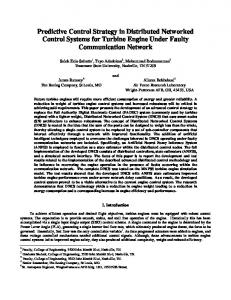
Figure 4. Transient response of the IM drive using MOPSO-MPC controller for the first speed track assuming load torque disturbance. The load torque is stepped up from 0.0 Nm to 50 Nm at t = 2 s.

disturbance compensation [34]. In the first speed trajectory, the speed of the IM is kept at zero for 0.1 s and then the speed increased to 500 rpm in 0.5 s, and then the motor speed is kept constant at this value during the next 2.5 s. The load torque is stepped up from 0.0 Nm to 50 Nm at t = 2 s. It has been observed that the speed command and actual motor speed are adjusted and good tracking performance has been accomplished utilizing MOPSO-MPC. A small speed plunge is seen at the moment of load disturbance; however, the motor speed is reestablished very rapidly. Figures 4–6 illustrate the dynamic performance of the MPC-MOPSO control strategy and the MPC-SOPSO versus the conventional PI controllers. Clearly, the PI controller has poor dynamic performance, particularly during the starting condition, and it is significantly influenced when a load disturbance is implemented. The MPC-MOPSO has been tried likewise at different speed commands, including negative speed, very low speed, and zero speed. In the second speed trajectory, the machine starts from zero speed increased straight to 500 rpm at time t = 0.6 s, and then the speed is kept constant until t = 1 s. At that point the speed of the IM is decelerated back to zero at t =1.6 s and then the speed is kept steady at zero until t = 2 s, and then the speed is accelerated in the reverse direction straight to –500 rpm at t = 2 .6 s. The speed is 2978

ELGAMMAL and EL-NAGGAR/Turk J Elec Eng & Comp Sci

Stator current (A)

2000 1500 1000 500 0 -500

Speed (RPM)

600 400 200 0 -200

Electromagnetic Torque (Nm)

800 600 400 200 0 -200

DC BUS(V)

1200 1000 800 600 400 200 0

Flux

0.8 0.6 0.4 0.2 0

0

0.5

1

1.5

2

2.5

3

Figure 5. Transient response of the IM drive using PID controller for the first speed track assuming load torque disturbance. The load torque is stepped up from 0.0 Nm to 50 Nm at t = 2 s.

Rotor Speed (rpm)

515 510 505 500 495 PID Controller SOPSO-MPC MOPSO-MPC

490 485 480 0.5

1

1.5

Time (s)

2

2.5

3

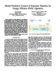
Figure 6. Comparison of speed dynamic responses for the first speed track with step load disturbance (the load torque is stepped up from 0.0 Nm to 50 Nm at t = 2 s) based on the proposed MOPSO-MPC, SOPSO-MPC, and PI controllers. Zooming for different instances at 0.5 and 2.0 s.

then kept constant at –500 rpm until t = 3 s. The load torque is suddenly applied from zero to 50 Nm at t = 2 s. Figures 7–9 demonstrate the comparison of the dynamic performance utilizing the MPC-MOPSO, MPC2979

ELGAMMAL and EL-NAGGAR/Turk J Elec Eng & Comp Sci

Stator current (A)

2000 1500 1000 500 0 -500 -1000

Speed (RPM)

1000 500 0 -500 -1000

Electromagnetic Torque (Nm)

1000 500 0 -500

DC BUS(V)

1500 1000 500 0 1 0.8 0.6 0.4 0.2 0

Flux

0

0.5

1

1.5

2

2.5

3

Figure 7. Transient response of the IM drive using MOPSO-MPC controller for the second speed track assuming load torque disturbance. The load torque is stepped up from 0.0 Nm to 50 Nm at t = 2 s. Stator current (A)

2000 1500 1000 500 0 -500

Speed (RPM)

600 400 200 0 -200 -400 -600

Electromagnetic Torque (Nm)

1000 500 0 -500

DC BUS(V)

1200 1000 800 600 400 200 0

Flux

0.8 0.6 0.4 0.2 0 0

0.5

1

1.5

2

2.5

3

Figure 8. Transient response of the IM drive using PI controller for the second speed track assuming load torque disturbance. The load torque is stepped up from 0.0 Nm to 50 Nm at t = 2 s.

2980

ELGAMMAL and EL-NAGGAR/Turk J Elec Eng & Comp Sci

520 Rotor Speed (rpm)

510 500 490 480

PID Controller SOPSO-MPC MOPSO-MPC

470 460 450 0.5

0.6

0.7

0.8 Time (s)

0.9

1

1.1

Rotor Speed (rpm)

10 5 0 -5

PID Controller SOPSO-MPC MOPSO-MPC

-10 -15 1.5

1.55

1.6

1.65

1.7

1.75

1.8

1.85

1.9

1.95

2

Time (s)

Rotor Speed (rpm)

-450 PID Controller SOPSO-MPC MOPSO-MPC -500

-550 2.5

2.55

2.6

2.65

2.7

2.75 Time (s)

2.8

2.85

2.9

2.95

3

Figure 9. Comparison of speed dynamic responses for the second speed track with step load disturbance (the load torque is stepped up from 0.0 Nm to 50 Nm at t = 2 s) based on the proposed MOPSO-MPC, SOPSO-MPC, and PI controllers. Zooming for different instances at 0.6, 1, 1.6, and 2.6 s. Stator current (A)

2000 1500 1000 500 0 -500 -1000

Speed (RPM)

1000 500 0 -500 -1000

Electromagnetic Torque (Nm)

2000 1500 1000 500 0 -500 -1000

DC BUS(V)

1500 1000 500 0 1 0.8 0.6 0.4 0.2 0 0

Flux

0.5

1

1.5

2

2.5

3

Figure 10. Transient response of the IM drive using MOPSO-MPC controller for the third speed track assuming load torque disturbance. The load torque is stepped up from 0.0 Nm to 50 Nm at t = 2 s.

2981

ELGAMMAL and EL-NAGGAR/Turk J Elec Eng & Comp Sci

Stator current (A)

2000 1500 1000 500 0 -500

Speed (RPM)

600 400 200 0 -200 -400 -600

Electromagnetic Torque (Nm)

1000 500 0 -500

DC BUS(V)

1200 1000 800 600 400 200 0

Flux

0.8 0.6 0.4 0.2 0

0

0.5

1

1.5

2

2.5

3

Figure 11. Transient response of the IM drive using PI controller for the third speed track assuming load torque disturbance. The load torque is stepped up from 0.0 Nm to 50 Nm at t = 2 s.

Rotor Speed (rpm)

-300 PID Controller SOPSO-MPC MOPSO-MPC

-350 -400 -450 -500 -550 1.9

2

2.1

2.2

2.3 Time (s)

2.4

2.5

2.6

2.7

Rotor Speed (rpm)

500 400 300 200 PID Controller SOPSO-MPC MOPSO-MPC

100 0 -100

0.05

0.1

0.15

0.2

0.25

0.3

0.35

0.4

0.45

0.5

Figure 12. Comparison of speed dynamic responses for the third speed track with step load disturbance (the load torque is stepped up from 0.0 Nm to 50 Nm at t = 2 s) based on the proposed MOPSO-MPC, SOPSO-MPC, and PI controllers. Zooming for starting and step load instances at t = 2 s.

2982

ELGAMMAL and EL-NAGGAR/Turk J Elec Eng & Comp Sci

SOPSO, and PI controllers. It has been demonstrated that the proposed MPC-MOPSO controller has better dynamic performance and has accomplished the steady-state value very rapidly. Although there is some speed variety, the speed comes back to its typical level rapidly when the step-load torque is applied, showing solid effectiveness against load torque disturbance while the PI controller showed a bad performance particularly at starting conditions and at the moment of load disturbance or speed change. Additionally, the dynamic response of the proposed MPC-MOPSO controller has been tested using MPC-MOPSO and PI controllers utilizing a sinusoidal speed trajectory with 500 rpm amplitude and the load torque is suddenly increased from no load to 50 Nm at t = 2 s. Figures 10–12 demonstrate that an excellent tracking response has been accomplished using the MPC-MOPSO control strategy in spite of the load torque disturbance. The results illustrate the capacity of MPC-MOPSO to accurately follow the sinusoidal speed track and to handle the load torque disturbance. Interestingly, unmistakably poor transient performance is connected with the PI controller in the beginning period and when load aggravation is connected at t = 2 s. A THD and error performance comparison is given in the Table for the proposed MOPSO-MPC controller, SOPSO-MPC controller, and conventional PI controller. From the results given in the Table, it is evident that the proposed MOPSO-MPC can improve the performance of the IM and lessen the effects of load and speed disturbances. It is clear that the THD of the stator current is reduced from 7.76% (using the conventional PID controller) and 3.65% (using the SOPSO-MPC controller) to 1.79% (using the MOPSO-MPC controller), which is below the mark of 5% specified in the IEEE-519 standard. The proposed MOPSO-MPC controller has yielded the lowest THD (1.79%) and has better performance as compared with the other controllers. Table. System performance comparison.

Control technique Speed error (%) THDi (stator current) Torque ripple (%) THDv (inverter voltage) THD DC bus voltage DC bus voltage error %

Conventional PID controller 7.76% 6.18% 7.26% 5.16% 8.12% 5.76%

SOPSO-MPC

MOPSO-MPC

3.65% 2.93% 3.75% 3.02% 4.08% 4.05%

1.79% 1.24% 2.59% 1.16% 2.14% 2.09%

7. Conclusion This paper has effectively exhibited the utilization of a new control approach based on MPC-MOPSO for optimal control of constrained sensorless vector control of an induction motor, which is utilized as a part of a FC-battery-superconductor EV. A set of multiobjective functions has been handled using the proposed MPCMOPSO while respecting the provided drive system constraints appointed to the load torque, the magnetic flux, the DC voltage, and the motor speed. The effectiveness of the proposed MPC-MOPSO optimization control approach has been assessed at different operating speeds and load torque conditions such as forward, reverse, very low, high speed, and sinusoidal speed track and a load torque disturbance was applied for each speed command with machine parameter variations. The simulation results carried out by MATLAB/Simulink demonstrated that the proposed MPC-MOPSO controller has a better dynamic response and better tracking of speed trajectory at all speeds than both the SOPSO and PI controllers. The proposed MPC algorithm can achieve satisfactory performance when appropriate parameters are chosen and tuned using MOPSO and hence this can be applied to large fields of industrial process controllers. 2983

ELGAMMAL and EL-NAGGAR/Turk J Elec Eng & Comp Sci

References [1] Abdallah T, Mamadou BC, Brayima D, Yacine A. DC/DC and DC/AC converters control for hybrid electric vehicles energy management: ultracapacitors and fuel cell. IEEE T Ind Inform 2013; 9: 686-696. [2] Thounthong P, Pierfederici S, Martin JP, Hinaje M, Davat B. Modeling and control of fuel cell/supercapacitor hybrid source based on differential flatness control. IEEE T Veh Technol 2010; 59: 2700-2710. [3] Camara MB, Dakyo B, Gualous H. Supercapacitors and battery energy management based on new European driving cycle. Journal of Energy and Power Engineering 2012; 6: 168-177. [4] Ahmed ZD, Vladimir P. Vector controlled induction motor drive based on model predictive control. In: 11th International Conference on Actual Problems of Electronics Instrument Engineering; 2–4 October 2012; Novosibirsk, Russia. pp. 167-173. [5] Jose T, Jayendra T, Kamalesh H, Krishna V. An improved scheme for extended power loss ride-through in a voltagesource-inverter-fed vector-controlled induction motor drive using a loss minimization technique. IEEE T Ind Appl 2016; 52: 1500-1508. [6] Jaroslaw G, Haitham A. Speed sensorless induction motor drive with predictive current controller. IEEE T Ind Electron 2013; 60: 699-709. [7] Andrew S, Shady G, John F. Improved rotor flux estimation at low speeds for torque MRAS-based sensorless induction motor drives. IEEE T Energy Conver 2016; 31: 270-282. [8] Yaman Z, Shady G, David A. Model predictive MRAS estimator for sensorless induction motor drives. IEEE T Ind Electron 2016; 63: 3511-3521. [9] Xiaodong S, Long C, Zebin Y, Huangqiu Z. speed-sensorless vector control of a bearingless induction motor with artificial neural network inverse speed observer. IEEE-ASME T Mech 2013; 18: 1357-1366. [10] Francesco A, Tommaso C, Filippo D, Adriano F, Antonino S. Convergence analysis of extended Kalman filter for sensorless control on induction motor. IEEE T Ind Electron 2015; 62: 2341-2352. [11] Habibullah MD, Dylan DL. A speed-sensorless FS-PTC of induction motors using extended Kalman filters. IEEE T Ind Electron 2015; 62: 6765-6778. [12] Mousavi-Aghdam SR, Sharifian MBB. Nonlinear adaptive observer for sensorless control of induction motor. In: 20th Iranian Conference on Electrical Engineering; 2012: Tehran, Iran. pp. 376-379. [13] Yung-Chang L, Chen-Lung T, Wen-Cheng P, Cheng-Tao T. Full-order stator flux observer based sensorless vector controlled induction motor drives applying particle swarm optimization algorithm. In: International Symposium on Computer, Consumer and Control; 4–6 July 2016; Xi’an, China. pp. 899-902. [14] Patel C, Ramchand R, Sivakumar K, Das A, Gopakumar K. A rotor flux estimation during zero and active vector periods using current error space vector from a hysteresis controller for a sensorless vector control of IM drive. IEEE T Ind Electron 2011; 58: 2334-2344. [15] Lascu C, Boldea I, Blaabjerg F. A class of speed-sensorless sliding mode observers for high-performance induction motor drives. IEEE T Ind Electron 2009; 56: 3394-3403. [16] Zaky MS. Stability analysis of speed and stator resistance estimators for sensorless induction motor drives. IEEE T Ind Electron 2012; 59: 858-870. [17] Boglietti A, Cavagnino A, Lazzari M. Computational algorithms for induction-motor equivalent circuit parameter determination—Part I: Resistances and leakage reactances. IEEE T Ind Electron 2011; 58: 3723-3733. [18] Ko J, Choi J, Chung D. Hybrid artificial intelligent control for speed control of induction motor. In: International Joint Conference SICE-ICASE; 18–21 October 2006; Busan, South Korea. pp. 678-683. [19] Ji ZC, Shen YX. Back-stepping position control for induction motor based on neural network. In: 1st IEEE Conference on Industrial Electronics and Applications; 24–26 May 2006; Singapore. New York, NY, USA: IEEE. pp. 1-5.

2984

ELGAMMAL and EL-NAGGAR/Turk J Elec Eng & Comp Sci

[20] Lin FJ, Shieh HJ, Shyu KK, Huang PK. On-line gain tuning IP controller using real coded genetic algorithm. Electr Pow Syst Res 2004; 72: 157-169. [21] Khalil M, Ahmed E, Mohamed R. Model predictive control using FPGA. International Journal of Control Theory and Computer Modeling 2015; 5: 1-14. [22] Sivakumar R, Shennes M. Design and development of model predictive controller for binary distillation column. International Journal of Science and Research 2014; 5: 445-451. [23] Holkar K, Waghmare L. An overview of model predictive control. International Journal of Control and Automation 2010; 3: 47-63. [24] Thomsen S, Hoffmann N, Fuchs F. PI control, PI-Based state space control and model-based predictive control for drive systems with elastically coupled loads-a comparative study. IEEE T Ind Electron 2011; 58: 3647-3657. [25] Mapok K, Zuva T, Masebu H, Zuva K. Performance comparison of two controllers on a nonlinear system. International Journal of Chaos, Control, Modelling and Simulation 2013; 2: 17-30. [26] Bayoumi EHE, Awadallah MA, Soliman HM. Deadbeat performance of vector-controlled induction motor drives using particle swarm optimization and adaptive neuro-fuzzy inference systems. Electro-motion Scientific Journal 2011; 18: 231-242. [27] Ryohei S, Fukiko K, Hideyuki I, Chikashi N, Yoshikazu F, Eitaro A. Automatic tuning of model predictive control using particle swarm optimization. In: Proceedings of the IEEE Swarm Intelligence Symposium; 2007. New York, NY, USA: IEEE. pp. 221-226. [28] Sofiane B, Mohammed C, Fouad A, Salim F. A new approach for fuzzy predictive adaptive controller design using particle swarm optimization algorithm. Int J Innov Comput I 2013; 9: 3741-3758. [29] Ngatchou P, Zarei A, El-Sharkawi A. Pareto multi objective optimization. In: Proceedings of the 13th International Conference on Intelligent Systems Application to Power Systems; 6–10 November 2005. pp. 84 -91. [30] Berizzi A, Innorta M, Marannino P. Multiobjective optimization techniques applied to modern power systems. In: IEEE Power Engineering Society Winter Meeting; 2001. New York, NY, USA: IEEE. pp. 1503-1508. [31] Coello CA, Lechuga MS. MOPSO: A proposal for multiple objective particle swarm optimization. In: Proceedings of the 2002. Congress on Evolutionary Computation, Part of the 2002 IEEE World Congress on Computational Intelligence; May 2002. New York, NY, USA: IEEE. pp. 1051-1056. [32] Jihane K, Mohamed C. Optimization of hybrid renewable energy power systems using evolutionary algorithms. In: 5th International Conference on Systems and Control; 25–27 May 2016; Marrakesh, Morocco. pp. 383-388. [33] Fawzan S, Mohamed A. Model predictive control for deadbeat performance of induction motor drives. WSEAS Transactions on Circuits and Systems 2015; 14: 304-312. [34] Finn H. Comparing PI tuning methods in a real benchmark temperature control system. Norwegian Society of Automatic Control, Modeling, Identification and Control 2010; 31: 79-91.

2985