unsupervised non-parametric Bayesian models fit to the segmentation task will be in ..... and "want to" contractions (c) and (d) below are grammatical, but not (e).
MORPHOLOGICAL SEGMENTATION USING DIRICHLET PROCESS BASED BAYESIAN NON-PARAMETRIC MODELS
A THESIS SUBMITTED TO THE GRADUATE SCHOOL OF INFORMATICS OF MIDDLE EAST TECHNICAL UNIVERSITY
SERKAN KUMYOL
IN PARTIAL FULFILLMENT OF THE REQUIREMENTS FOR THE DEGREE OF MASTER OF SCIENCE IN COGNITIVE SCIENCE
FEBRUARY 2016
Approval of the thesis:
MORPHOLOGICAL SEGMENTATION USING DIRICHLET PROCESS BASED BAYESIAN NON-PARAMETRIC MODELS
submitted by the degree of
SERKAN KUMYOL in partial ful�llment of the requirements for Master of Science in Cognitive Science, Middle East Technical
University by,
Prof. Dr. Nazife Baykal Director,
Graduate School of Informatics
Assist. Prof. Dr. Cengiz Acartürk Head of Department,
Cognitive Science, METU
Prof. Dr. Cem Boz³ahin Supervisor,
Cognitive Science, METU
Assist. Prof. Dr. Burcu Can
Department of Computer Engineering, Hacettepe University Co-supervisor,
Examining Committee Members: Prof. Dr. Deniz Zeyrek Boz³ahin Cognitive Science Department, METU Prof. Dr. Cem Boz³ahin Cognitive Science Department, METU Assist. Prof. Dr. Burcu Can Department of Computer Engineering, Hacettepe University Assist. Prof. Dr. Cengiz Acartürk Cognitive Science Department, METU Assist. Prof. Dr. Murat Perit Çak�r Cognitive Science Department, METU
Date:
I hereby declare that all information in this document has been obtained and presented in accordance with academic rules and ethical conduct. I also declare that, as required by these rules and conduct, I have fully cited and referenced all material and results that are not original to this work.
Name, Last Name:
Signature
iii
:
SERKAN KUMYOL
ABSTRACT
MORPHOLOGICAL SEGMENTATION USING DIRICHLET PROCESS BASED BAYESIAN NON-PARAMETRIC MODELS
Kumyol, Serkan M.S., Department of Cognitive Science Supervisor
: Prof. Dr. Cem Boz³ahin
Co-Supervisor
: Assist. Prof. Dr. Burcu Can
February 2016, 54 pages
This study, will try to explore models explaining distributional properties of morphology within the morphological segmentation task. There are di�erent learning approaches to the morphological segmentation task based on supervised, semi-supervised and unsupervised learning. The existing systems and how well semi-supervised and unsupervised non-parametric Bayesian models �t to the segmentation task will be investigated. Furthermore, the role of occurrence independent and co-occurrence based models in morpheme segmentation will be investigated.
Keywords:
Natural Language Processing, Morphological Segmentation, Computa-
tional Linguistics, Dirichlet Process, Bayesian Non-Parametric Methods
iv
ÖZ
DRCHLET SÜREC TEMELL PARAMETRK OLMAYAN BAYES MODELLER LE MORFOLOJK BÖLÜMLEME
Kumyol, Serkan Yüksek Lisans, Bili³sel Bilimler Program� Tez Yöneticisi
: Prof. Dr. Cem Boz³ahin
Ortak Tez Yöneticisi
: Assist. Prof. Dr. Burcu Can
ubat 2016 , 54 sayfa
Bu tezde, morfolojik bölümleme içerisindeki da§�l�m özelliklerini aç�klayan modeller incelenecektir. Morfolojik bölümlemeye, gözetimli, yar� gözetimli ve gözetimsiz ö§renmeyi temel alan çe³itli ö§renim yakla³�mlar� mevcuttur. Bu çal�³mada, mevcut sistemleri inceleyerek, parametrik olmayan yar� gözetimli ve gözetimsiz Bayes'ci yakla³�mlar�n bölümleme i³lemine ne kadar uygun oldu§unu gözlemleyece§iz. Ek olarak, morfolojik bölümlemede, morfemleri birbirinden ba§�ms�z ve ba§�ml� olarak ele alan modellerin rolleri incelenecektir.
Anahtar Kelimeler: Do§al Dil i³leme, Morfolojik Bölümleme, Hesaplamal� Dilbilim, Dirichlet Süreci, Parametrik Olmayan Bayes Modelleri
v
I dedicate my thesis to whom I love and many friends. My mother Tayyibe Yontar always supported me in my decisions and never gave up on me. My sister Sevcan Kumyol Yücel made me feel safe and con�dent during my entire study. The my beloved one Ece O§ur was my candle in the night that enlightened my path. I should also mention about my gratitude to my aunt Sema Kumyol Ridpath who supported me during my entire education.
vi
ACKNOWLEDGMENTS
I would like to express my deepest gratitude to my supervisor, Dr.
Cem Boz³ahin.
He motivated and encouraged me to pursue academics even when I felt lost during the research. More importantly, he gave me an understanding of scienti�c approach. Thanks to him, now I feel more con�dent and competent to move forward into science by knowing that I still need much to do and much to learn. Without my co-supervisor Dr. Burcu Can's guidance, patience and endless belief in me, this thesis could not be �nished. I would like to thank her for introducing me to the topic as well for the support on the way. She contributed to the study in many ways. The main idea of the study and methodology were architectured by her. She also helped me to overcome with the major challenges of the study. The knowledge I gained from her is precious and invaluable. I am grateful to Dr. Deniz Zeyrek who teached me background theories. I also would like to thank to Dr. Cengiz Acarturk who �rstly introduced me to machine learning. Dr. Murat Perit Çak�r always encouraged and positively motivated me. In addition, I would like to thank the many contributors in my thesis, who have willingly shared their precious knowledge during the study.
I especially would like to
thank to my colleagues, brahim Hoca, Gökçe O§uz, Ay³egül Tombulo§lu and Murathan Kurfal� for their contributions. My cousin Adam Sinan Ridpath also supported me during the study. I would like to thank my loved ones, who have supported me throughout the entire process.
vii
TABLE OF CONTENTS
ABSTRACT
. . . . . . . . . . . . . . . . . . . . . . . . . . . . . . . . . . . . .
iv
ÖZ . . . . . . . . . . . . . . . . . . . . . . . . . . . . . . . . . . . . . . . . . . .
v
ACKNOWLEDGMENTS
. . . . . . . . . . . . . . . . . . . . . . . . . . . . . .
vii
TABLE OF CONTENTS
. . . . . . . . . . . . . . . . . . . . . . . . . . . . . .
viii
LIST OF TABLES . . . . . . . . . . . . . . . . . . . . . . . . . . . . . . . . . .
xi
LIST OF FIGURES
. . . . . . . . . . . . . . . . . . . . . . . . . . . . . . . . .
xii
LIST OF ABBREVIATIONS . . . . . . . . . . . . . . . . . . . . . . . . . . . .
xiii
CHAPTERS
1
INTRODUCTION
1
1.1
Introduction
. . . . . . . . . . . . . . . . . . . . . . . . . . . .
1
1.2
Role of Statistical Approaches in LA . . . . . . . . . . . . . . .
3
1.2.1
. . . . . . . . . . . . .
5
. . . . . . . . . . . . . . . . . . . . .
6
1.3.1
Frequentist vs. Bayesian Approach to Reasoning . . .
6
1.3.2
LOTH
. . . . . . . . . . . . . . . . . . . . . . . . . .
7
1.4
Aim of The Study . . . . . . . . . . . . . . . . . . . . . . . . .
8
1.5
Scope . . . . . . . . . . . . . . . . . . . . . . . . . . . . . . . .
9
1.3
2
. . . . . . . . . . . . . . . . . . . . . . . . . . . . .
Statistical Approaches to LA
Motivation of The Study
BACKGROUND
. . . . . . . . . . . . . . . . . . . . . . . . . . . . . .
viii
11
2.1
Introduction
. . . . . . . . . . . . . . . . . . . . . . . . . . . .
11
2.2
Linguistic Background . . . . . . . . . . . . . . . . . . . . . . .
11
2.2.1
Morphology
. . . . . . . . . . . . . . . . . . . . . . .
11
2.2.2
Approaches to Morphology . . . . . . . . . . . . . . .
12
2.2.2.1
Split-Morphology Hypothesis
12
2.2.2.2
Amorphous Morphology Hypothesis
2.2.2.3
2.3
2.4
. . . . . . .
. . .
12
Item-and-Arrangement and Item-and-Process Morphology . . . . . . . . . . . . . . . . .
13
2.2.3
Morphemes as Syntactic Elements . . . . . . . . . . .
14
2.2.4
Turkish Morphology . . . . . . . . . . . . . . . . . . .
15
2.2.4.1
Orthography of Turkish
15
2.2.4.2
Morphophonemic Process
. . . . . . . . . .
. . . . . . . . .
16
Machine Learning Background . . . . . . . . . . . . . . . . . .
18
2.3.1
Bayesian Modeling
. . . . . . . . . . . . . . . . . . .
18
2.3.2
Parameters and Conjugation . . . . . . . . . . . . . .
19
2.3.3
Dirichlet Distribution . . . . . . . . . . . . . . . . . .
20
2.3.4
Multinomial Distribution . . . . . . . . . . . . . . . .
20
2.3.5
Bayesian Posterior Distribution
. . . . . . . . . . . .
21
2.3.6
Inferring Multinomial Dirichlet
. . . . . . . . . . . .
21
2.3.7
Bayesian Non-Parametric Modeling . . . . . . . . . .
22
2.3.8
Chinese restaurant process (CRP) . . . . . . . . . . .
23
2.3.9
Hierarchical Dirichlet Process
. . . . . . . . . . . . .
24
. . . . . . . . . . . . . . . . . . . . . . . . . . . . . .
25
Markov Chain Monte Carlo (MCMC) . . . . . . . . .
25
Inference
2.4.1
ix
2.4.1.1
3
26
. . . . . . . . . . . . . . . . . . . . . . . . . . . . . . . . .
27
3.1
Introduction
. . . . . . . . . . . . . . . . . . . . . . . . . . . .
27
3.2
Statistical Models of Learning of Morphology . . . . . . . . . .
27
3.2.1
Letter Successor Variety (LSV) Models . . . . . . . .
27
3.2.2
MDL Based Models . . . . . . . . . . . . . . . . . . .
29
3.2.3
Maximum Likelihood Based Models . . . . . . . . . .
31
3.2.4
Maximum A Posteriori Based Models . . . . . . . . .
32
3.2.5
Bayesian Parametric Models . . . . . . . . . . . . . .
33
3.2.6
Bayesian Non-parametric Models
. . . . . . . . . . .
34
. . . . . . . . . . . . . . . . . . .
35
METHODOLOGY AND RESULTS
4.1
Introduction
. . . . . . . . . . . . . . . . . . . . . . . . . . . .
35
4.2
Allomorph Filtering . . . . . . . . . . . . . . . . . . . . . . . .
35
4.3
Unigram Model
. . . . . . . . . . . . . . . . . . . . . . . . . .
36
4.4
HDP Bigram Model . . . . . . . . . . . . . . . . . . . . . . . .
39
4.5
Inference
41
4.6
Results and Evaluation
4.7
5
. . . . . .
LITERATURE REVIEW ON UNSUPERVISED LEARNING OF MORPHOLOGY
4
Metropolis-Hastings Algorithm
. . . . . . . . . . . . . . . . . . . . . . . . . . . . . .
. . . . . . . . . . . . . . . . . . . . . .
42
4.6.1
Experiments With Unsupervised Models
. . . . . . .
43
4.6.2
Experiments With Semi-supervised Models . . . . . .
43
Comparison With Other Systems
. . . . . . . . . . . . . . . .
46
. . . . . . . . . . . . . . . . .
47
Future Work . . . . . . . . . . . . . . . . . . . . . . .
48
CONCLUSION AND FUTURE WORK
5.0.1
x
LIST OF TABLES
Table 2.1
Partial Paradigm of Finnish Noun
Table 2.2
Phoneme alternations of Turkish
Table 3.1
Input Words
Table 3.2
Stem Table
talo
'house'. . . . . . . . . . . . .
14
. . . . . . . . . . . . . . . . . . . .
16
. . . . . . . . . . . . . . . . . . . . . . . . . . . . . . .
29
. . . . . . . . . . . . . . . . . . . . . . . . . . . . . . . .
29
Table 3.3
Su�x Table . . . . . . . . . . . . . . . . . . . . . . . . . . . . . . . .
29
Table 3.4
Encoded words . . . . . . . . . . . . . . . . . . . . . . . . . . . . . .
30
Table 4.1
Results from unsupervised unigram model . . . . . . . . . . . . . . .
43
Table 4.2
Results from unsupervised bigram HDP model
. . . . . . . . . . . .
43
Table 4.3
Results from semi-supervised unigram model
. . . . . . . . . . . . .
44
Table 4.4
Results from semi-supervised bigram HDP model . . . . . . . . . . .
44
Table 4.5
Comparison of our semi-supervised model with other algorithms with
supervised parameter tuning participated in Morpho Challenge 2010 for Turkish . . . . . . . . . . . . . . . . . . . . . . . . . . . . . . . . . . . . . .
Table 4.6
46
Comparison of our unsupervised model with other unsupervised sys-
tems in Morpho Challenge 2010 for Turkish
xi
. . . . . . . . . . . . . . . . .
46
LIST OF FIGURES
Figure 2.1
Plate Diagram of DP . . . . . . . . . . . . . . . . . . . . . . . . . .
23
Figure 2.2
An illustration of CRP
. . . . . . . . . . . . . . . . . . . . . . . . .
24
Figure 2.3
An illustration of HDP . . . . . . . . . . . . . . . . . . . . . . . . .
25
Figure 2.4
Diagram of Metropolis-Hastings Algorithm . . . . . . . . . . . . . .
26
Figure 3.1
Word split points in a LSV model . . . . . . . . . . . . . . . . . . .
28
Figure 3.2
A sample morphology with signature pointers and tables, taken from
Goldsmith (2006)
. . . . . . . . . . . . . . . . . . . . . . . . . . . . . . . .
31
Figure 4.1
An overview of the model
. . . . . . . . . . . . . . . . . . . . . . .
36
Figure 4.2
The plate diagram of the unigram model . . . . . . . . . . . . . . .
38
Figure 4.3
The plate diagram of the bigram HDP model
. . . . . . . . . . . .
39
Figure 4.4
Comparison of Results From Unigram Models
. . . . . . . . . . . .
44
Figure 4.5
Comparison of Results From Bigram Models . . . . . . . . . . . . .
45
Figure 4.6
Comparison of Results With The Highest F-measure
45
xii
. . . . . . . .
LIST OF ABBREVIATIONS
1
First Person
ACC
Accusative
ART
Article
AI
Arti�cial Intelligence
BTP
Backward Transitional Probability
CCG
Combinatory Categorial Grammar
CRP
Chinese Restaurant Process
DEM
Demonstrative
DP
Dirichlet Process
FTP
Frontward Transitional Probability
HDP
Hierarchical Dirichlet Process
HMM
Hidden Markov Model
HTP
High Transitional Probability
INST
Instrumental
LA
Language Acquisition
LOC
Locative
LOTH
Language of Thought
LSV
Letter Successor Variety
LTP
Low Transitional Probability
MAP
Maximum a Posteriori
MCMC
Markov Chain Monte Carlo
MDL
Minimum Description Length
ML
Maximum Likelihood
MLE
Maximum Likelihood Estimation
N
Noun
NLP
Natural Language Processing
OBJ
Object
PAS
Predicate-Argument Structure
PAST
Past tense
PCFG
Probabilistic Context-free Grammar
PLU
Plural
PMF
Probability Mass Function
xiii
POS
Poverty of Stimulus
POSS
Possessive
PRE
Pre�x
SBJ
Subject
SF
Shannon-Fano Method
Sing
Singular
SV
Successor Variety
UG
Universal Grammar
xiv
CHAPTER 1
INTRODUCTION
1.1
Introduction
The term and
morphology derives from the Greek word "morph-," meaning shape or form,
morphology
means the study of form(s). A well-known de�nition of morphology is
the study of the internal structure of words. Researchers have been scienti�cally curious about understanding words since the �rst morphologist, Panini, who formulated the 3,959 rules of Sanskrit morphology in the 4th century BCE in the text "Astadhyayi" using a constituency grammar. The question of why morphology is so important could be answered by stating that if we need to understand the ultimate building blocks of the universe, we need to look at atoms, or in other words, its constituents. In the case of agglutinating language, these blocks are morphemes, the smallest meaning-bearing units of language. Morphological forms have a signi�cant e�ect on phonology, syntax, and semantics in productive languages, as the operations in linguistic morphology have powers of deriving new word forms and in�ecting words. To learn such languages, one needs to acquire a substantive set of rules for morphosyntax (Hankamer, 1989).
In linguistics, morphology refers to the mental system involved in word formation, the internal structure of words and how they are formed (Arono� and Fudeman, 2011, p.
opened is formed open and the su�x ed. The phonological realization of individual morphemes is called as morph. Morphs in Turkish occur with alternations
2). Words consist of stems and a�xes; for example, the English word by the concatenation of the stem
in vowels; for example, Turkish pluralization has two di�erent morphs with the back vowel
a, çocuk-lar
�children� and the front vowel
e, ev-ler
�houses�. Vowel alternations
in Turkish are de�ned by a set of rules, which will be mentioned in section 2.2.4. We call morphemes with allomorphic forms
allomorphs, these are morphemes carrying the
same semantic information of their class with vowel alternations.
In this study, we
assume that the stems are free morphs that occur freely, while the su�xes must be bounded and called boundary morphemes. Our focus on Turkish language arises from its productivity and morphologically rich nature. There are challenges regarding Turkish in terms of its morphological analysis. Controversially, morphologically simpler languages like English could be modeled in terms of word-based approaches due to their lack of productivity. Unlike agglutinating languages, in English, word forms could be stored in a word-based lexicon. Turkish has a large amount of word forms that cannot be stored in a word-based lexicon.
1
Furthermore, theoretically there could be in�nite numbers of meaningful morpheme sequences in Turkish. The number of possible word forms that one can construct is in�nite due to recursion.
Recursion in Turkish is caused by morphemes that derive
causative verbs and relative adjectives. One examples of the productivity of Turkish is described below: Example 1.1: OSMANLILATIRAMAYABLECEKLERMZDENMSNZCESNE Where boundaries of morphemes are: OSMAN-LI-LA-TIR-AMA-YABL-ECEK-LER-MZ-DEN-M-SNZ-CESNE where the -'s indicate the morpheme boundaries. The adverb in this example can be translated into English as "(behaving) as if you were of those whom we might consider not converting into an Ottoman." (O�azer et al., 1994, p.2) The diversity of morphological forms and syntactic rules in agglutinating languages causes a sparse distribution of forms. Turkish is a solid example of rich morphological diversity and productivity. In this study, the segmentation of Turkish morphology is motivated by a semi-supervised model with orthographic rules for allomorphs adopted as prior information.
As a result, we aim to make use of Turkish allomorphy in
clustering of phonological forms. From a cognitive perspective, the importance of morphology arises in the acquisition of morphemes. When learning agglutinating languages, acquisition is a task of learning diverse morphological forms, classes, and their interactions. The learning of morphology entails segmenting words into morphemes. While there is evidence that word boundaries are learned during language acquisition (LA) of infants (Thiessen and Sa�ran, 2003), there is insu�cient evidence about phonological and prosodic dimensions of the learning processes. In addition to the evidence about the signi�cance of morphology in LA, the acquisition of morphemes includes a language-speci�c task unlike the universal grammar (UG) suggests. Several studies have provided evidence of the language-speci�c impact of nominal and verbal in�ections on LA (Slobin, 1985; Bittner et al., 2003). These studies revealed that nominal in�ections and verbal in�ections di�ered in the developmental process of infants. This suggests that, LA is not dominated by innate structures; there is room for language-speci�c information and exposure more than UG suggests. If the distributional properties of di�erent languages have an impact on linguistic levels, understanding their distributions may provide us with a basic understanding of how morphologically rich languages are acquired. Statistical language modeling methods are based on machine learning methodologies categorized under three learning systems: First, in supervised learning, the system trains on a set of labelled corpus to identify the target function. Training data consist of the input and output values, whereby the system predicts unseen data with the function it inferred from the tagged data.
It is di�cult to tag all morphological phenomena
of agglutinating languages like Turkish and overcome with computational expense. Furthermore, due to the high amount of possibility of a large amount of unseen data, training procedure of the model mostly underestimate possible word forms.
Unlike
supervised learning, the unsupervised and semi-supervised machine learning systems,
2
are more likely to be independent of extra information. However, in semi-supervised learning, training is motivated by extra information which is not be found in the training set, while unsupervised models do not require any other information but untagged training data. A computational model made of semantic information combined with the logical forms could explain a language beyond semi-supervised and unsupervised computational models for natural languages, the main concern about such models, arises from the computational expense. Çak�c� et al. (2016), reported results from the wide-coverage parser that consist of a semantically rich lexicon with lexicalized grammars involving. As a result of modeling lexicon paired with logical form or predicate-argument structure (PAS), training the parser with rich head informations improved parsing accuracy. Furthermore, the wide-coverage parsing with lexicalized grammars achieved to parse a wide range of constructions in Turkish, which no other parser able cover such wide-range of unique constructions. The wide-coverage parsing with such lexicon model proved itself to be a feasible model in contrary to computational concerns. Natural language processing (NLP) applications are capable of processing language independently, but language-speci�c information needs to be involved within the process in order to obtain a better performing model. This study is to incorporate languagespeci�c knowledge and the distributional properties of Turkish morphology from a form-driven perspective. Form-driven models may be de�cient in covering the morpholinguistic properties of language, but they give us clues about the distributional properties of morphology and boundary detection involvement in the acquisition of morphology. Additionally, as much as language learning explained unsupervised, the assumptions rely on innateness involve less. This study focuses on non-parametric Bayesian models for morphological segmentation and language learning.
Our method di�ers
from other non-parametric Bayesian models of Turkish by embedding orthographic rules into the clustering process where both bigram and unigram models involved. Therefore, our research questions are as follows:
1. How much of learning could be explained in terms of form-driven non-parametric Bayesian models, and is the word form enough to supervise the learning process? 2. Does supervising a non-parametric Bayesian model with orthographic rules as prior information result in better segmentations?
1.2
Role of Statistical Approaches in LA
The capability of LA is unique among human beings, as we have the ability to manipulate our linguistic knowledge and establish complex structures within the boundaries of our grammars, even in the absence of su�cient prior knowledge. Pinker (1995) demonstrated how the combinatorial rule system of human language is unique compared to other animals. Every human being is the master of her/his native language, regardless of his/her intelligence, DNA, race, etc. Humans are able to compose word forms by manipulating grammars of their languages unlike non-human animals. The acquisition of language, therefore, is the most mysterious topic in the cognitive sciences.
3
There are two mainstream approaches to LA. One is the nativist approach, in which LA is considered as cognitive resource that is an innate UG
(Chomsky, 1965). UG
suggests that all humans have a set of rules which are common to all natural languages.
These rules are innate and can be updated (or reduced) in correspondence
to the language children are exposed to.
One supportive hypothesis is the Poverty
of Stimulus (POS) argument (Chomsky, 1975). The POS argument suggests that it is impossible to acquire a language by exposure in the absence of negative evidence. The negative evidence here is correction of ungrammatical forms by adult speakers. The lack of negative evidence, expected to cause over-generalization in the language learning process. When an infant begins to learn a language, learning turns into the problem of narrowing down the set of UG into input language. Evidence shows that babies achieve a stable state even when there is a a lack of corrections in primary linguistic data (PLD) (Gleitman and Newport, 1995). This suggests that humans have a system that is more sophisticated than what they are being exposed to. Another argument supported by the nativist approach is the problem of ambiguity, which is related to the POS argument. For a baby, sentences (a) and (b) below are not problematic; they can acquire these syntactic constructs even there is lack of negative evidence in the environment (Crain and Pietroski, 2001). a)
John washed himself.
b)
John said that he thinks Bill should wash himself.
Again Crain and Pietroski (2001, p.7) argued: " So why do not children acquire a more permissive grammar, according to which 'himself ' may depend on 'John' in (b), But if children allow multiple interpretations - e.g, the antecedent of 'himself ' can be any prior term no positive evidence would prove them wrong." This evidence leads to the conclusion that humans have prior knowledge of the principle of the
binding theory :
a re�exive pronoun must be locally bound.
Regarding the learning of linguistic constraints, the nativist point of view suggests that constraints are also an innate capability of human beings. For example, the "wanna" and "want to" contractions (c) and (d) below are grammatical, but not (e). Children do not overgeneralize language due to their innate capacities. c)
I wanna go to school.
d)
I want you to go school.
e) *I
wanna you to school.
According to the continuity hypothesis (Pinker, 1991; Crain and Thornton, 1998), even when children make mistakes, they will never go beyond the boundaries of UG. The mistake of a child is a meaningful grammatical construction of another language because UG covers all possible human languages. Pinker (1995, p.157) suggested, "That is, before children have learned syntax, they
4
know the meaning of many words, and they might be able to make good guesses as to what their parents are saying based on their knowledge of how the referents of these words typically act (for example, people tend to eat apples, but not vice versa )." If children can extract extralinguistic information before they start talking, negative evidence could still be out there, which could contradict the POS argument.
The computational approach to the concept of UG that argued by Cowie (1999) is in a more empiricist state, which presumes that exposure is more essential than innate knowledge in language acquisition. Cowie (1999) also suggested that there is an innate device in LA, but she also suggested that there is a computational process involved in it. Computational modeling of language is a useful approach to understand how much of LA can be explained in terms of exposure and innate knowledge.
1.2.1 Statistical Approaches to LA Signi�cant evidence of experience-dependent LA arises from Sa�ran et al. (1996), a research with eight month-old babies. The main aim of the research is to reveal how babies acquire language even in cases of a lack of exposure and to study the role of statistical cues on a child's learning capacity. To simulate exposure, a familiarization process applied that contains information about the target arti�cial language syntax without any other cues (pitch-accent, boundaries, prosodic components, phonetics, etc.).
The experiment started with exposing babies to arti�cial language.
In the
second minute of exposure, babies were able to distinguish novel and familiar orderings of three-syllable strings.
Furthermore, children can detect word and part-word
boundaries by a longer period of exposure. Results suggest that, at least in early LA, experience plays an important role in acquiring transitional probabilities between parts of words. Pelucchi et al. (2009) in their research, implemented the research method in Sa�ran et al. (1996) to natural languages. Two counterbalanced languages; Italian and Spanish are choosen as the experiment languages, instead of the arti�cial languages. Furthermore, eight-month-old native English monolingual infants were exposed to Italian and Spanish.
Unlike Sa�ran et al. (1996), the eye gazing duration was used as the
measurement method. Test items were distinguished by their backward transitional probabilities (BTP) and front transitional probabilities (FTP). The front and backward probabilities de�ne the direction of adjacent syllables. Two identi�ers, the low transitional probability (LTP) and high transitional probability (HTP), were used to measure child's sensitivity to their perception of LTPs and HTPs of words. The results (ibid.) revealed that children's sensitivity to BTP is signi�cantly independent of the language group to which they belong. Additionally, children are capable of computing both FTP and BTP, but BTP has more coverage on data due to the structural properties of the babies' natural language. Another approach by Wong et al. (2012) employed extra-linguistic information within perspective of grounded LA with respect to the evidential foundation of Carpenter et al. (1998) which, suggests that children who engage in joint attention with caregivers tend to have a faster learning process. The extra-linguistic input incorporated utterances, gaze, touch, etc. features, with the task of reducing the process to a proba-
5
bilistic context-free grammar (PCFG) learning, where syntax is sensitive to transitional probabilities. As result of this approach, the model allowed them to reveal the relationship between acquisition tasks in the study. Results revealed that it is important to use ideal learning models when investigating LA, and incorporating social cues with linguistic information could provide us important information about the signi�cance
1
of the extra-linguistic features in learning . Lany et al. (2007) �rstly, criticize the role of statistical cues in LA; their approach pointed to early language studies that were mainly nativist, due to a lack of knowledge about the distributional properties of languages.
The study, focused on the
arti�cial languages used in LA research and concluded that even though such models are arguable about their representational capacity of natural languages, but they provide a useful framework to understand LA. Arti�cial languages can be manipulated to observe and understand the e�ect of di�erent transitional probabilities in learning without isolation from correlation with infants' prior knowledge. Lany et al. (2007) concluded that there is some computational processing in LA, but the features of the method and the method itself are still a mystery. The transitional probabilistic approach, chunking, and n-gram models do not fully explain or provide a comprehensive understanding of learning by themselves; therefore, further wide-coverage models should be developed to understand LA from a computational perspective.
1.3
Motivation of The Study
The aim of computational models of language is to model the language learning process based on certain assumptions. This study presumes that computational models may not correspond to the mind's internal structures, but they could represent and manipulate given data with respect to researcher's belief about the process to be modeled. Furthermore, computational modeling provides us knowledge to hypothesize how LA happens and a framework where empirical knowledge uni�es with beliefs. Certain theories, hypotheses, and assumptions have been developed for to modeling of the data. In this section, �rstly, internalist and frequentist reasoning methodologies of the modeling will be presented. Secondly, language of thought hypothesis (LOTH) (Fodor, 1975) presented as a foundational argument for cognitive models of mind. We neither oppose nor suggest an alternative hypothesis to LOTH. The only semantic dimension involved in this study is the semantic assumptions about Turkish phonology, such as allomorphy. We aim to discover how far morphology can be learned from the syntactic forms on the phonological dimension. With incorporating allomorphic information to our model, we aim to get a better clustering of phonological forms.
1.3.1 Frequentist vs. Bayesian Approach to Reasoning There are two approaches to the statistical reasoning of data that in�uence modeling. The �rst approach is the frequentist analysis of data, which presumes that data are su�cient to understand themselves. The second approach is the internalist (Bayesian) 1
child's eye (encoded as child.eye which represent gaze directions of child) is the most extra-
linguistic information in learning.
6
view, suggesting that beliefs and prior knowledge should be involved in the analysis of data. The frequentist approach proposes that no subjective beliefs are involved in knowledge, but data are the knowledge itself, and observations could be measured from experimental results, with the perspective of "let data speak for themselves." However, in modeling we need to extract more knowledge than data and �xed parameters. The main di�erence between Bayesian and frequentist approaches is how probability is used to understand the data. Frequentists use probability with the purpose of data sampling. The Bayesian approach uses probability more widely to model both sampling and prior knowledge. The internalist (Bayesian) approach proposes that the probability is in a person's degree of belief about an event, not an objective measurement, as suggested by the frequentist approach. Lilford and Braunholtz (1996, p.604) argued that: " when the situation is less clear cut (...
)
conventional statistics may
drive decision makers into a corner and produce sudden, large changes in prescribing. The problem does not lie with any of the individual decision makers, but with the very philosophical basis of scienti�c inference." This suggests that the classic statistical approaches may not necessarily be involved in the analysis of uncertain cases. Instead, Bayesian inference should be used for inferring knowledge due to its degrees of freedom for uncertainty. Geisler and Kersten (2002) suggested that the human visual capacity is best modeled in terms of Bayesian models in contrast to frequentist models. The computational studies of Marr (1982) and the evolutionary studies of Pinker (1997) are examples that are well explained and uni�ed by the Bayesian framework. Bayesian inference is a �ne graded reasoning framework for the philosophy of science with room for subjective information. Bayesian likelihood models can construct, eliminate, or hypothesize beliefs about data. Experiences, innate abilities, and beliefs are observable in human predictions, and the Bayesian reasoning has degrees of freedom to represent them within a likelihood model.
Modeling the
capability of the Bayesian approach also provides room for uncertainty.
Humans'
decision-making falls under uncertainty when trying to predict actions with insu�cient data. Under uncertain conditions, human beings rely on their prior knowledge and try to decide which actions to perform based on experience. Learning a concept updates prior knowledge about certain conditions to reduce uncertainty.
This probability is
called subjective probability, which could successfully model uncertainty with Bayesian methods (Dagum and Horvitz, 1993).
1.3.2 LOTH While form-driven approaches to language learning are limited by syntax, LOTH claims that the cognitive processes are combinatorial systems in which tokens are represented with both syntactic and semantic information as functions of syntactic tokens. Thus, any computational system aiming to model LA as a cognitive process needs to be governed by both syntax and semantic functions of syntactic tokens. LOTH (Fodor, 1975) assumes that thought and thinking occur in a mental language.
If there was
not a �rst language that enables language learning, the learning would fall into in�nite regress. The LOTH is a system of representations in which representations are physically realized in the brains of the thinkers. The LOTH presumes that thought
7
is a token of a representation that has a syntactic (constituent) structure combined with its related semantics.
Thus, thinking is a cognitive process in which combina-
torial operations de�ned over representations are causally sensitive to the syntactic representations (tokens), in other words, thoughts have combinatory behaviour. The LOTH is a hypothesis about the nature of thought and thinking that consist a family of ideas; causal-syntactic theory of mental processes (CSMP) and the representational theory of mind (RTM), about the way we represent our world.
CSMP
attempt to explain mental processes as causal processes de�ned over the syntax of mental representations and RTM claims, these mental representations have both syntactic structure and a compositional semantics.
Therefore, thinking takes place in
language of thought (LOT). There are 3 main arguments for the LOTH: First, the LOT acquires the form of language, instead of imitating the grammar of a speci�c language. According to the hypothesis, the brain is capable of doing high-level abstractions so it can encode di�erent formal communication methods and symbolic systems. Second, symbolic language is not equivalent to UG, but a common way of thinking and linguistic structure in all human thought. Fodor (1975) suggested that learning a language requires an internal mental language common to all human beings. Third, thinking is an abstract highlevel process. While thinkers may have an idea about their thinking, there is no such access to the LOT. Only representations that are being tokened and the manipulation processes are visible to thinkers. The LOT is an innate device beneath manipulation and tokenizing that enables the manipulation of representations.
Thus, the compu-
tational models of language learning are can not be one-to-one correspondent with mentalese but they try do deduce it from the logical form and the phonological form. Unlike arti�cial languages, natural languages are accommodate uncertainty that, makes it harder to model with computational systems. But the LOTH provides degrees of freedom for computationalism, since both approaches are presume that, the concepts prevents learning from in�nite regress are primitive. The point of computational models is to deduce the hidden layer between form with meaning, namely, grammar. Recent developments on arti�cial intelligence (AI) and formal logic, gives LOTH explanatory power within a naturalistic framework. Alan Turing's idea of a Turing Machine and Turing computability provides room for combination of computationalism with the LOTH. Turing's well-known experiment; the Turing test suggests that if a conversational agent (computational machine) is indistinguishable from a human being, then that machine would be an intelligent agent.
According to LOTH, a combinatorial
system with primitives would be a part of machinery of conversational agent.
1.4
Aim of The Study
The main aim of this study is to explore the cognitive plausibility of form-driven semi-supervised non-parametric Bayesian models with allomorphic priors in the morphological segmentation task. By adding orthographic rules as prior information, we aim to compare the results of the semi-supervised model with those of the unsupervised model to understand whether language-speci�c knowledge (allomorphic priors) has a signi�cant e�ect on the segmentation task. Additionally, the a�ect of incorporating
8
morpheme co-occurrences into a form-driven computational model will be explored.
1.5
Scope
The scope of this study is Turkish words together with orthographic rules for morphological forms. Clustering morphemes as allomorphs may give us a better understanding of the learning process.
9
CHAPTER 2
BACKGROUND
2.1
Introduction
This chapter presents the linguistic and machine learning background used in this study to give a better understanding of methodologies to the reader. is organized into two sections:
The chapter
section 2.2 presents the linguistic background that
involves the general concepts in morphology, syntax, and phonology with examples, and section 2.3 focuses on the machine learning background that our model is based on.
2.2
Linguistic Background
This section focuses on the linguistic knowledge essential to the segmentation task. The knowledge we will present is about morphology and its interaction with phonology and syntax.
2.2.1 Morphology As stated in section1.1, the term morphology is the study of the smallest meaningbearing elements of a language, morphemes. Morphology is also an interface between phonology and syntax, where morphological forms as constituents carry both syntactic and phonetic information. In productive languages like Finnish, Turkish, Tagalog, and Hungarian, morphemes can derive new word forms and modify the meaning of a word form. Thus, a�xation in such languages causes words to have a complex internal structure.
Productive
languages contain a set of rules for morphological composition that are able to generate a considerable amount of word forms by the concatenation of morphemes (Hankamer, 1989).
Example 2.2.1 The word certain can have di�erent word forms when combined with grammatical morphemes, as in the case of the words
uncertain, certainty, uncertainty
Morphologically productive languages are called agglutinating languages. There are also languages without any morphology in which words consist of syllables, like Chi-
11
nese, Vietnamese, and Mandarin, which are called
isolating languages.
2.2.2 Approaches to Morphology This section presents some of the classical theories essential to morphology:
the
split morphology hypothesis, the amorphous morphology hypothesis, the item-and-
1
arrangement and item-and-process morphology .
2.2.2.1 Split-Morphology Hypothesis According to the split morphology hypothesis developed by Anderson (1982, 1992), Matthews (1972, 1991), and Perlmutter (1988), derivational morphology is too irregular to be combined with in�ectional morphology; thus, they belong to separate components of grammar. Derivation is handled by lexical rules, while (regular) in�ection is handled by syntactic rules. In this study, the segmentation task does not aim to distinguish between any in�ectional and derivational morphemes, thus, they are treated as the same element.
2.2.2.2 Amorphous Morphology Hypothesis In the amorphous morphology hypothesis, Anderson (1992) proposed that word structure is the output of an interaction between grammatical areas, and therefore it can not be localized to a single morphological component. According to this hypothesis, word structures cannot be explained merely by the concatenation of morphemes, but they can be explained by rule-governed relations among words with respect to the phonological internal structure assigned to words and eliminating morphologically motivated boundary elements. Amorphous morphology de�nes signi�cant distinctions between in�ection, derivation, and compounding, in terms of their place in a grammar.
w
w
Anderson exempli�ed his idea with the well-known Wakashan language K ak 'ala. every sentence is verb-initial, and some in�ectional morphemes of noun phrases are not attached to constituents of the phrase, but instead to the verb, as shown in example 2.2.2 (from Anderson (1992)).
Example 2.2.2 nanaq[@]sil-ida
i?g[@]lâwat-i
[@]liwinuxwa-s-is
Guides-SBJ/ART
expert-DEM
hunter-INST-his
mestuwi harpoon
migwat-i seal-DEM 1
For more recently presented two dimensional approach see Stump (2001).
12
la-xa PRE-OBJ/ART
" An expert hunter guides the seal with his harpoon."
Anderson (1992, p.19) further analysed the sentence as follows: "It is clear that if the
w
w
morphology of K ak 'ala is responsible for characterizing the internal form of phonological words, it will have to overlap heavily with the syntax in order to describe such facts. An alternative, however, is to suggest that the phonological word is not actually the domain of morphological principles of word structure." His theory of phonology and morphology naively involves into our work through analyzing surface forms according to the orthographic rules of Turkish, which we will describe in the upcoming sections.
2.2.2.3 Item-and-Arrangement and Item-and-Process Morphology The morphological debate of mapping phonological forms to morphosyntactic forms was �rst identi�ed by Hockett (1954).
The item-and-arrangement hypothesis: both
roots and a�xes are treated as morphemes, item-and-process: roots are morphemes, but a�xes are rules. These theories are the models for the mapping between phonological form and morphosyntactic information. Item-and-process theories propose that a word is the result of an operation (morphosyntactic rules) applied to a root with some morphosyntactic features, which modi�es the phonological form of syntactic unit. Example 2.2.3 shows a word formation rule for the application of the Turkish plural su�x sults in a phonological sequence of the single word
kitap-lar.
-lar to a noun stem kitap 'book' rekitaplar instead of the composition
Example 2.2.3 Word Formation Rule for Plural [
+N
[
+PLU
/X/
] ]
→/
Kitap
→
X/ Kitaplar
As presented in example 2.2.3, item-and-process morphology takes a morpheme as input and applies it to a stem, resulting in a new sequence of phonemes that cannot be broken into morphosyntactic parts.
In item-and-arrangement theories, words are considered as a set of morphemes consisting of a root a�xed by a morpheme.
In this model, sets are sequences made of
phonological correspondences of roots and morphemes, as shown in example 2.2.4:
Example 2.2.4 kitaplar → kitap +lAr root [+PLU]
13
Table 2.1: Partial paradigm of Finnish noun
talo
'house'. From Roark and Sproat
(2007, p.64). category
Sing.
Plu
Nominative
talo
talo-t
Genitive
talo-n
talo-j-en
Partitive
talo-a
talo-j-a
Inessive
talo-ssa
talo-j-ssa
Elative
talo-sta
talo-j-sta
Adessive
talo-lla
talo-j-lla
Ablative
talo-lta
talo-j-lta
Allative
talo-lle
talo-j-lte
Both theories are used frequently in morphology; the item-and-process approach was defended recently by Arono� (1993), and item-and-arrangement theory accounted for the theory of distributed morphology (Halle and Marantz, 1993). Furthermore, Roark and Sproat (2007) also mentioned how both theories of morphology are suitable for di�erent languages. For example, highly in�ected languages, such as Classical Greek and Sanskrit, in which morphological rules are better explained in terms of word structure because of the rich information-carrying a�xes.
In this case, a�xation is
not simply a concatenation, but a�xing a particular variant of the stem, this process also depends on the particular paradigm of a stem. Roark and Sproat (2007) also suggested that agglutinating languages, such as Finnish and Turkish, which have a systematical morphosyntax in a linear order, can be modeled in terms of morphemes rather than rules. Finnish word
talo
reproduced at 2.1 exempli�es the regularities and irregularities (un-
derlined forms) of Finnish nominal morphology. The irregular exceptions among plural a�xes can be treated by encoding alternations as either conditional case selection in plural morphemes (-i/-j vs. -t) or de�ning two allomorphs, one with variant
-t
(in case
of a NOMINATIVE a�x) other with -i/-j variants. Therefore, a systematic agglutinating language like Finnish can be explained in terms of item-and-arrangement. While Turkish is a morphologically complex language, morphotactics is clear enough to be explained in terms of �nite state machines (O�azer et al., 1994).
2.2.3 Morphemes as Syntactic Elements As an example of multiple representations of allomorphs; the allomorph ish represents the forms -lar and -ler of plural su�xes.
-lAr
in Turk-
Unifying morphemes into
allomorphs is a process of applying Turkish vowel alternation rules to the phonemes, with respect to the roundness and backness of the preceding vowel. The high productivity of morphology presented in example 1.1, consists of free and bounded morphemes.
Free morphemes most likely to occur freely, while bounded
morphemes must be a�xed to another morpheme.
abling
formed by morphemes -
dis, -able
and
14
For instance, in the case of
-ing, -able
is the
dis-
root and free morpheme
pre�x and -ing su�x. Roots are free morstem can not be broken into further
of the word and other morphemes -dis is a
phemes that can not be further analyzed while a
parts. We can observe this di�erence clearly in compound words .
Example 2.2.5.
The word form
board.
skateboard
is a stem consists of two roots
skate
and
su�x, pre�x, in�x circum�x depending on their position of the concatenation to a stem.
Furthermore, bound morphemes belong to di�erent classes like and
Example 2.2.6. and
-able
The word
decomposable
consists of
-de
as pre�x
compose
as stem
as su�x.
Tuwali Ifugao, the language of the Philippines, uses circum�xes.
baddan-gan 'helpfulness', -baddang 'help'.
formed by
ka�an
For example,
ka-
, a nominalizer circum�x and the verb
Morphemes belong to small and closed classes, e.g., articles, locatives, and genitives, and occur more frequently than the words of open classes. Morphemes have a complex semantic relation with words from lexical categories, and are syntactically more predictable, by a deterministic �nite state machine Turkish morphosyntax (O�azer et al., 1994).
2.2.4 Turkish Morphology A�xation process of Turkish, mostly occurs as the concatenation of su�xes to a stem, root, or another su�x, while pre�xes are rarely seen. There is a range of su�xes in phonological terms, and allomorphs di�er on the basis of their vowel harmony. Surface forms of morphemes are often processed by morphophonemic operations for the grammatical construction of words. The grammatical composition of morphemes requires some morpho-phonological processes to ensure agreement between the a�xed morpheme and the preceding vowel on the basis of
vowel harmony.
Under certain
conditions, deletion, alternation, and drop rules on roots and morphemes are initiated; these rules are called morphophonemic operations that are part of morphophonemic processes.
2.2.4.1 Orthography of Turkish The Turkish alphabet consists of 29 characters: 8 vowels: a, e, �, i, o, ö, u and ü; and 21 consonants: b, c, ç, d, f, g, h, j, k, l, m, n, p, r, s, ³, t, v, y, and z. Vowels can be grouped to accumulate vowel harmony:
15
Table 2.2: Phoneme alternations of Turkish. (from O�azer et al. (1994)) 1. D : voiced (d) or voiceless (t) 2. A : back (a) or front (e) 3. H : high vowel (�, i, u, ü) 4. R : vowel except o, ö 5. C : voiced (c) or voiceless (ç) 6. G : voiced (g) or voiceless (k)
1. Back vowels: {a, �, o, u} 2. Front vowels: {e, i, ö, ü} 3. Front unrounded vowels: {e, i} 4. Front rounded vowels: {ö, ü} 5. Back unrounded vowels: {a, �} 6. Back rounded vowels: {o, u} 7. High vowels: {�, i, u, ü} 8. Low unrounded vowels: {a, e}
O�azer et al. (1994) used meta-phonemes to describe the two-level morphology of Turkish, which we used in our allomorph �ltering algorithm to map phonemes to allomorphs. The phoneme alternations are shown in Table 2.2 are used for alternations in vowels, for example,
-lar.
�lAr
is the allomorph for plural stands for both plural su�xes
-ler
and
Meta-phonemes provides a useful notation for the two-level realization of allo-
morphs consisting of
surface form and lexical form.
Example 2.2.7. Lexical form:
bulut-lAr N(cloud)-PLU
Surface form:
bulut0lar
bulutlar
Where -lAr represents the plural su�xes for two cases of metaphoneme A: the back vowel
a
or the front vowel
e.
One of them is chosen according to Turkish vowel harmony
rules.
2.2.4.2 Morphophonemic Process In Turkish, allomorphs are essential in the concatenation process, and variable vowels of an allomorph are called metaphonemes.
Metaphonemes consist of six characters
representing related vowels, as shown in Table 2.2.
16
Rules of alternation depend on
vowels and their orthographic rules. Rules for vowel harmony are described as examples in which capital letters are metaphonemes of allomorphemes. '0' is the notation for deleted phonemes and morpheme boundaries. In this study, rules are included in the segmentation model by a �ltering algorithm for vowels. Processes on consonants aim to cluster Turkish morphological forms into allomorphic representations. The rules for vowel alternations are as follows:
Example 2.2.8.
Low-unrounded vowels: If the last vowel of the preceding morpheme
a.
is a back vowel, metaphoneme A alternates to
Lexical form:
arkada³-lAr
N(friend)-PLU
Surface form:
arkada³0lar
arkada³lar
Lexical form:
ayna-lAr
N(mirror)-PLU
Surface form:
ayna0lar
aynalar
Example 2.2.9 Low-unrounded vowels:
If the last vowel of the preceding morpheme
is a front vowel, metaphoneme A alternates to
Lexical form:
çiçek-lAr
N(�ower)-PLU
Surface form:
çiçek0ler
çiçekler
Lexical form:
bebek-lAr
N(baby)-PLU
Surface form:
bebek0ler
bebekler
Example 2.2.10 High vowels:
If the last vowel of the preceding morpheme is a back-
rounded, metaphoneme H alternates to
u 2.
Lexical form:
ko³ul-Hm
N(term)-1SG-POSS
Surface form:
ko³ul0um
ko³ulum
Lexical form:
macun-Hm
N(paste)- 1SG-POSS
Surface form:
macun0um
macunum
Lexical form:
ko³-Hyor-yHm
N(run)-POSS
Surface form:
ko³0uyor00um
ko³uyorum
Example 2.2.11 High vowels:
If the last vowel of the preceding morpheme is a front-
rounded vowel, metaphoneme H alternates to
2
e.
Lexical form:
üzüm-Hm
Surface form:
üzümm0üm
Lexical form:
göz-Hm
ü
N(grape)-1SG-POSS üzümüm N(eye)-1SG-POSS
cases § and ç excluded from our research due to our data does not contain any form with that
characters.
17
Surface form:
göz0üm
gözüm
Example 2.2.12 High vowels:
If the last vowel of the preceding morpheme is a
�
back-unrounded vowel, metaphoneme H alternates to
Lexical form:
gitar-Hm
N(guitar)-1SG-POSS
Surface form:
gitar0�m
gitar�m
Lexical form:
zaman-Hm
N(time)- 1SG-POSS
Surface form:
zaman0�m
zaman�m
Example 2.2.13 High vowels:
If the last vowel of the preceding morpheme is a front-
unrounded vowel, metaphoneme A alternates to
i
Lexical form:
zafer-Hm
N(victory)-1SG-POSS
Surface form:
zafer0im
zaferim
Example 2.2.14 Consonant mutation: tation rule also known as consonants,
p, ç, t, k,
voicing,
is concatenated with a su�x starting with a vowel consonants,
voiceless consonant alternates to
biça k
b, c, d, g
biça g -im
knife
In Turkish, according to consonant mu-
if a morpheme ending with one of the voiceless respectively.
kita p
knife -1.SG.POSS
kita b -i
book
'my knife'
book -ACC
'the book'
Example 2.2.15 Consonant assimilation:
If a morpheme starting with consonant
D (see Table 2.2 for alternation rules) concatenates with a morpheme ending with one of the voiceless consonants
yaprak leaf
p, ç, t, k, g, h, s, ³, f
yaprak- t a
aç
leaf -LOC
open
'at leaf '
2.3
alternates to a
t
or
d.
aç -t � open -PAST 'opened'
Machine Learning Background
2.3.1 Bayesian Modeling 3 expresses actual knowledge about the model parameters. A 4 Bayesian probabilistic model is a parametrized joint distribution over variables. In The Bayesian modeling
3
Bayesian modeling originates from Bayes theorem.
Bayes theorem was proposed by Thomas
Bayes (c. 1702 �17 April 1761), an English mathematician. 4 Typically interpreted as a generative model of the data.
18
Bayesian modeling, the actual model aims to infer posterior distribution
p(θ|D),
the
probability of new parameters given data:
p (θ | D) =
where probability distribution
p (θ)
p (D | θ) p(θ) p(D)
over the parameters is named
(2.1)
prior distribution.
For incoming data, the probability of information they contain is expressed with respect
likelihood
p (D | θ) which is proportional to the distribution of the observed data given the model parameters and the p(D) is marginal probability. The marginal probability of data is the probability calculated through all to model parameters named the
of data
possible values of data used for normalization. Bayes' theorem uses the likelihood and the prior to de�ne the inverse probability distribution over parameters. the data called
The inverse probability distribution of parameters of
posterior probability.
Posterior probability is the revised probability
of parameter values occurring after taking into consideration the incoming data. To calculate the probability of new data, the theorem uses prior and likelihood. There are two cases according to the type of parameters: continuous or discrete:
p (D) =
X
p (D | θi )p(θi )
(2.2)
p (D | θ) p(θ)dθ
(2.3)
i Continuous parameters:
Z p (D) =
Bayesian modeling de�nes the probability of an instance with respect to parameter
5 or hypotheses. A Bayesian model is either parametric or non-
values, latent variables
parametric. The Bayesian parametric models are the Bayesian models with pre-de�ned parameters, we can call their parameters are constants de�ned by model designer. The Bayesian non-parametric models has countably in�nite parameters that grows with the data.
2.3.2 Parameters and Conjugation Integration over parameters bypasses the possibility of the biased estimation of parameters by integrating all possible values of the parameters. For example, if we have a set of segmentations
S
of a corpus
C
and latent variables are the segmentation points:
Z p (S | C) = here
θ
p (S | C, θ) p (θ | C) dθ
(2.4)
is a set of parameters that are integrated out without being estimated.
By
integrating the parameters out, all possible values are carried out for the inference of latent variables without any estimation. The integration over parameters leads a more comprehensive inference of latent variables. 5
We integrate out the latent varibles without estimating them.
19
When we adopt Bayesian modeling, the prior probability over parameters can be de�ned. A de�ned prior is also called a
conjugate prior when the posterior distribution
has the same form as the prior distribution. For example, Gaussian distribution is self-conjugating by the Gaussian likelihood function, so if we choose Gaussian prior distribution, the posterior will be in Gaussian form. In the case of multinomial distribution, it has a conjugate prior in the form of Dirichlet distribution. The conjugation of a multinomial distribution with a Dirichlet prior results in a posterior distribution with a Dirichlet distribution form. De�ning a multinomial distribution on de�ne
{1, . . . . . . . . . , N }
hyperparameters.
tion when we assume that
possible outcomes and setting
θ
helps us to
Here hyperparameters are parameters of prior distribu-
θ
is following some prior distribution.
distribution prior, we can say that
β
is a hyperparameter for
For the Dirichlet
θ.
xi ∼ M ultinomial(θ)
(2.5)
θ ∼ Dirichlet(β) The �rst line of equation states that with parameters
θ
xi
is drawn from a multinomial distribution
and in the second line states that, parameters
Dirichlet distribution with hyperparameters
θ
are drawn from a
β.
2.3.3 Dirichlet Distribution Dirichlet distribution is the multivariate generalization of the beta distribution. We can conceptualize Dirichlet distribution with a probability mass function (PMF). The randomness of a bag of dice with di�erent PMFs could be modeled with Dirichlet distribution. With respect to equation 2.5, Dirichlet distribution follows the form:
K 1 Y p (θ | β) = θkβk −1 B (β)
(2.6)
k=1
where
B (β)
is a normalising constant in a beta function form:
QK B (β) =
where
Γ
k = 1 Γ(βk )
Γ(
is the gamma function de�ned as
PK
k = 1 βk )
Γ(t)
(2.7)
= (t-1)! For positive integers.
2.3.4 Multinomial Distribution If we suppose that each datum in one of k possible outcomes with a set of probabilities
{x1 . . .xk }, multinomial models the distribution of the histogram vector that indicates 20
how many times each outcome is observed over N total number of data points.
K Y
N!
p (x | θ) = QK
k=1 nk ! k=1
θkxk
(2.8)
Where:
K X
N=
nk
(2.9)
k=1
Parameters
θk
are the probabilities of each data point
occurrences of data point
k
, and
nk
is the number of
xk .
2.3.5 Bayesian Posterior Distribution In a conjugate Bayesian analysis, we have a multinomial likelihood with the Dirichlet prior. After observing
nk
data, we have the posterior distribution for the parameters
as Can (2011, p.53) derived:
p (θ | x, β) ∝ p (x | θ) p (θ | β) N!
= QK
K Y
k=1 nk ! k=1
θkxk
K Y k = 1 Γ(βi ) θkβk −1 PK Γ( k = 1 βk ) k=1
QK
K Y k = 1 Γ(βi ) θknk +βk −1 PK n ! Γ( β ) k=1 k k = 1 i k=1 QK K Y N! k = 1 Γ(βi ) = QK θknk +βk −1 PK k=1 nk ! Γ( k = 1 βi ) k=1
N!
QK
= QK
∝ Dirichlet(nk + βk − 1) (2.10)
Equation 2.10 yields a Bayesian posterior in Dirichlet distribution form when we conjugate
β
distribution, multinomial and Dirichlet distribution.
2.3.6 Inferring Multinomial Dirichlet Can (2011, p.54) in her dissertation integrated out posterior mean using conjugacy as in equationCan 2.11:
21
Z p (xN +1 = j | x, β) =
(xN +1 = j | x, θ) (θ | β) dθ PK K Y Γ(N + k=1 βk θj Q K θknk +βk −1 dθ k=1 Γ(nk + βk ) k=1 PK Z K Y Γ(N + k=1 βk θj θj nj +βj −1 θknk +βk −1 dθ QK k=1 Γ(nk + βk ) k6=1 PK Z K Y n +β −1 Γ(N + k=1 βk θj nj +βj −1 θk k k dθ QK k=1 Γ(nk + βk ) k6=1 QK PK Γ(N + k6=1 Γ(nk + βk ) k=1 βk Γ(nj + βj + 1) PK QK Γ(N + k=1 βk + 1) k=1 Γ(nk + βk )
Z =
=
=
= =
nj + β j P N+ K k=1 βk
(2.11)
The posterior distribution of parameters in equation 2.11 are function as the prior distribution over the parameters.
This yielded a rich-get-richer behaviour, where if
previous observations of a given category are higher, then the next observation
xN +1
has a higher probability of being in the same category. If we consider both the probability of having a new category and of updating an existing category within an in�nite number of elements:
p (xN +1 = j | x, β) =
nj PK
j∈K N + k=1 βk βj otherwise PK N + k=1 βk
(2.12)
There are two probabilities: for incoming data either there is a new data point or it will belong to an existing category. The probability for a data point that is assigned to an existing category is proportional to the number of data points in that category. Otherwise, the probability would be proportional to the hyperparameter de�ned for that category.
This approach gives the advantage of natural smoothing for unseen
data by leaving a probability space for them.
2.3.7 Bayesian Non-Parametric Modeling Non-parametric models are models with an in�nite number of parameters, contrary to what the name suggests.
Dirichlet multinomial distribution consists of a �xed
number of parameters and observations, and it is not always likely to have that kind of data in nature. For example, in language processing, there are in�nite possibilities of morpheme segmentations in an agglutinating language like Turkish, as mentioned in Section 1.1.
Therefore, a
Dirichlet process
modeling data with in�nite parameters.
22
(DP) is a natural consequence of
Figure 2.1: Plate Diagram of DP
A DP is a distribution over distributions. Unlike Gaussian distributions, a DP has non�nite, dimensional, discrete random distributions. Therefore, the process is classi�ed as a non-parametric model. Dirichlet distribution allows �exibilities within data to be captured by its non-parametric stochastic structure.
G should be distributed according to Dirichlet distribution with ranΦ and α be a positive real number. Then for any �nite measurable partition A1 . . . . . . .An of Φ the vector (G (A1 ) , . . . . . . , G (An )) is random since G is random (Teh, 2010). G is DP distributed with a base distribution H and concentration parameter α therefore, the formula could be written as follows:
Every distribution
dom sampling. Let H be a distribution over
G ∼ DP (α, H) if (G (A1 ) , . . . . . . , G (Ar ))
∼
Dir(H (A1 ) , . . . . . . , αH(Ar )) (2.13)
Each
A
is generated from a
DP (α, H): Ai ∼ G
(2.14)
G ∼ DP (α,H) To obtain the probability distribution over
G,
which estimates future observations or
latent variables we need to integrate out as discussed in the section above. Integration is applied for a future observation
xN +1 = j
with Polya Urn Schemes (Blackwell and
MacQueen, 1973)
p (xN +1 = j | x, β) =
N 1 X α I (xi = j) + H(j) N +α N +α i=1
=
I
nj + αH(j) N +α
is an identity function that returns
0
when
xi 6= j ;
(2.15)
otherwise it returns
1.This
leads
us to a well-known de�nition of a DP, known as Chinese restaurant process (CRP).
2.3.8 Chinese restaurant process (CRP) The CRP is based on the de�nition of a restaurant with an in�nite number of tables and an in�nite number of seats, where each customer sits either at a new table or
23
Figure 2.2: An illustration of CRP
an existing one.
Each table has a unique menu to serve.
The customer chooses an
occupied table with a probability that is proportional to the number of customers who are already sitting at the table. If the chosen menu does not exist at any of the tables, the customer sits at a new table with a probability proportional to a de�ned constant
α.
While this process continues, tables with preferable menus will acquire a higher
number of customers. Thus, the rich-get-richer principle shapes the structure of the tables. As presented in Figure 2.2, if a customer
xn+1
sits at an existing table, the probability
will be de�ned by the number of customers already sitting at that table; otherwise, the probability will be calculated with respect to
α
and base distribution
major de�nitions of DP are the stick-breaking process
H (xn+1 ).Other
(Sethuraman, 1994; Ishwaran
and James, 2001) and the Pitman-Yor process (Pitman, 1995; Pitman and Yor, 1997).
2.3.9 Hierarchical Dirichlet Process The HDP consists of multiple DPs that are organized hierarchically with the DPs for all clusters sharing a base distribution, which itself is drawn from a DP. HDP is a dependency model for multiple DPs, which is more �exible than a single DP in uncovering group dependencies.
G0 ∼ DP (γ, H) Gj ∼ DP (α0 , G0 )
(2.16)
φji ∼ Gj xji ∼ F (φji ) Equation 2.16 completes de�nition of HDP (illustrated in �gure 2.3) where
G0
draws
F (φji ) stands for factors of single representations of given categories(j ). G0 ) this leads to a hierarchical structure where probability of a depends both on G and G0 .
from a DP and
G draws from DP(α , new customer
The HDP treats each incoming datum as a restaurant instead of customers, and for each restaurant, there are seats for customers at its tables.
The formula derived
from Polya Urn Schemes, still valid in the HDP case, but by de�nition probability of unseen restaurants with unseen customers, is calculated according to in �gure 2.3. distribution of
G0 ,
as shown
In the case of incoming data, it does not exist as a DP but as the
Gn ,
probability is proportional to concentration parameter
restaurant or customer does not exist, probability is calculated according to
24
α. G0 .
If a
Figure 2.3: An illustration of HDP
2.4
Inference
In machine learning, the inference of parameters plays a signi�cant role in estimation. While there are several approaches, like the maximum a posteriori (MAP) or maximum likelihood (ML), to perform the point estimation of parameters, we may need to estimate the posterior probabilities to understand the nature of parameters. Bayesian inference derives the posterior probability as a consequence of the prior probability and likelihood function.
The true nature of Bayesian inference needs an estimation
of the distributions over the possible values of the parameters. To estimate the parameters, we could use sampling by drawing random samples from their posterior distributions. Here we used the most common sampling method, Markov chain Monte Carlo (MCMC). The following section gives an intuition about this method.
2.4.1 Markov Chain Monte Carlo (MCMC) A Markov chain is a mathematical model for stochastic systems whose states are governed by a transition probability where an actual state only depends on a previous state. MCMC is a simulation technique used to determine the probability distributions in a complex model.
In MCMC, samples form a Markov chain where samples are
drawn randomly.
S = {S1 , S2 , . . . . . . . . . , S1 }
Let
be a set of states with respect to
their sequences:
p (Pn+1 = x | X1 = x1 , . . . . . . , Xn = xn ) = p (Pn+1 = x | Xn = xn )
(2.17)
25
2.4.1.1 Metropolis-Hastings Algorithm The Metropolis-Hastings algorithm was developed by- Metropolis et al. (1953) and generalized by Hastings (1970).
The Metropolis-Hastings algorithm, after drawing
random samples, determines whether to retain the sample according to an acceptance rule.
Figure 2.4: Diagram of Metropolis-Hastings Algorithm
The algorithm works on random draws from a distribution.
With each iteration,
the algorithm determines an accept/reject state with respect to the probability of parameters.
With each iteration, the algorithm gets closer to inducing the target
distribution from random samples.
26
CHAPTER 3
LITERATURE REVIEW ON UNSUPERVISED LEARNING OF MORPHOLOGY
3.1
Introduction
This section presents computational approaches to morphology and previous studies on non-parametric learning models. The present study covers morphological segmentation models based on the minimum description length (MDL), maximum likelihood estimation (MLE), maximum a posteriori(MAP), and parametric and non-parametric Bayesian approaches with a computational frame.
3.2
Statistical Models of Learning of Morphology
Statistical models are mathematical models consisting of equations that are actual beliefs about data. In the morphological segmentation task, the model learns morphology by mathematical equations and outputs the morphological analysis of a word. There are di�erent approaches to the segmentation task; in this section, some of the mainstream approaches are covered.
3.2.1 Letter Successor Variety (LSV) Models Successor variety (SV) was �rst proposed by Harris Harris (1955) as a segmenting method that transcribes spoken language utterances into morphemes. SV here is the number of letters that can follow each letter in a word. The main idea is counting letter successors for each letter to detect morpheme boundaries. If a letter has a signi�cantly high count of letter successors within an utterance, a new morpheme boundary is suggested.
Example 3.2.1
LSV would process an utterance
modeling
letter by letter, until the
model is unable to identify any boundaries due to the low letter successor count. Then, the actual count rises because of the number of possible morphemes (ie.
-ed )
already incremented letter successor points for letter
27
I.
-ing,
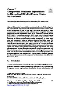
Figure 3.1: Word split points in a LSV model (taken from Can and Manandhar (2014))
Figure 3.1 visualizes splitting points as a tree structure where nodes are splitting points and branches address the letter sequences of splits. Harris manually de�ned
cuto�
val-
ues, which a�ect the segmentation points (bigger values cause the under segmentation of morphemes while lower values cause over segmentation). Following Harris (1955), LSV is used as a measure for the segmentation of words into morphemes (Hafer and Weiss, 1974; Déjean, 1998; Bordag, 2005; Goldsmith, 2006; Bordag, 2008; Demberg, 2007). Hafer and Weiss (1974) extended LSV by using predecessor and letter successor varieties to �nd segments and choosing the stem. Their approach suggests an improvement on LSV by replacing counts with entropies. Their study proposed four improvements on
cuto�, peak
and
plateau,
complete word and entropy. The entropy could be calcu-
lated as follows:
E (ki ) =
X Ck i Ck log 2 i Ckij P Ck i j
(3.1)
j ∈
k and E() is a function that returns letter k i . Cki is the total number of words in the corpus matching with the letter i of the word k and Ckij is the number of words in the corpus matching with the letter i with successor j. This approach has an advantage Where
i
is the letter pre�x of the word
successor entropy (LSE) of an a�x.
over earlier version because the LSE improves the morpheme boundary detection of morphemes with LSV counts. Déjean (1998) suggested another improvement on LSV method, such as three phases with a most frequent morpheme dictionary. The �rst step is to create a most frequent morpheme dictionary in which frequencies are obtained by LSV. The second phase involves using a morpheme dictionary to generate additional morphemes for words in the corpus, and the third phase is the �nal analysis on the corpus with a new morpheme dictionary. Bordag (2005) combined context information and LSV to reduce the noise and irregularities of LSV outputs.
The context information he used includes syntactic sim-
ilarity with respect to syntactic classes of words.
28
The �rst step is computing the
co-occurrences of adjacent words of a given word
W
by its log-likelihood.
The ob-
tained set of signi�cant adjacent words is called "neighborhood vectors." In his second step, he calculated the similarity of the vectors by common words within di�erent vectors and clustering.
Example. 3.2.2
painting cocoloring, walking, playing ), the highest number the words painting and playing is 70.
Considering a corpus of words in which the, word
occurs with a vector of words (paint, of adjacent di�erent word forms for
In his further research, Bordag (2006) used an algorithm consisting of two steps. The �rst step entails using the LSV; the second step is to insert analyzed words into a classi�er by morphemes and their frequencies. To analyze a word,
trie
trie 1
is searched until
the correct branches providing the right segmentations are revealed..
3.2.2 MDL Based Models MDL is an information theoretic model for the learning of morphology.
The MDL
principle was �rst introduced by Rissanen (1978), as in Occam's razor the best description of data or the best hypothesis is the one that leads to the best compression of the data. Grünwald (2005) made a clear statement: "[The MDL Principle] is based on the following insight: any regularity in a given set of data can be used to compress the data, i.e. to describe it using fewer symbols than needed to describe the data literally." The MDL theory is grounded on one-to-one correspondence between length functions and probability distributions. For a probability distribution bility measure
p (x)
is equal to
−log 2 p(x)
p
, the length of proba-
where it minimizes the expected description
length. From a Bayesian perspective, MDL can be used as the prior for model
argmin[−log 2 p (M | C)] = M
− log 2 [p (C | M ) p(M )] −log 2 [p(x)]
M:
(3.2)
∝ log 2 [p (C | M ) p(M )] Table 3.1: Input Words
Table 3.2: Stem Table
Table 3.3: Su�x Table
walk
referral
stem
code
su�x
code
walks
refer
walk
1
NULL
1
walked
refers
referr
2
s
2
walking
dump
refer
3
ed
3
referred
dumps
dump
4
ing
4
referring
preferential
preferenti
5
al
5
Brent et al. (1995) de�ned two models to solve the morpheme discovery problem: the �rst model is called simple recombination; it encodes a list of words with binary sequences of stems and su�xes in which the stems are kept in tables, as illustrated in 1
Look for Fredkin (1960) and Morrison (1968) for
29
trie.
stems guitar
su�xes
table
null
car
ed
book
ing
bottle
e
curse
s
the
es
glass Table 3.4: Encoded words Stem
Su�x
Stem
Su�x
00 00
00
01
110
01
100
00
00
100
100
01
00
101
101
00
01
100
101
01
01
101
1100
110
Tables 3.1, 3.2, 3.3, and 3.4. The most frequent stems and su�xes are encoded with shorter encodings. The optimal length of each code word is achieved by Shannon-Fano (SF) coding (Brent et al., 1995). Final segmentation is chosen when the morphological analysis results in a minimum code. Goldsmith (2001, 2006) proposed Linguistica, a state-of-the-art system for unsupervised morphology learning.
Linguistica uses signatures to encode the data, where
signature is a representation of the inner structure of a list of words that containing a�xes. Figure 3.2 presents the structure of a signature, where signatures are pointers for stems and su�xes. In addition, there are two more lists for stems and su�xes that contain letters. Here
M
is the morphology minimizing the objective function for the best morphology
in the corpus. The length of
M
gives information about the shortness of the morpheme
where this information is simplifying the decision of possible morpheme and the second term calculates how well the model �ts the corpus.
DescriptionLength (Corpus = C, M odel = M ) = length (M ) + log 2
1 p (C | M ) (3.3)
The log probability of a given word
w,
is analysed as belonging to given signature
σ
with stem t and su�x f, is as follows:
p (w = t + f ) = p (σ) p (t | σ) p (f | σ)
(3.4)
Another state-of-the-art system within the MDL principle is Morfessor, proposed
30
SimpleStem : car � N U LL SimpleStem : table s SimpleStem : guitar N U LL ed s ing
SimpleStem : book SimpleStem : bottle SimpleStem : curse � {SimpleStem : glass
N U LL es
{SimpleStem : the {N ull Figure 3.2:
A sample morphology with signature pointers and tables, taken from
Goldsmith (2006) tables are covering words: car, cars, table, tables, guitar, guitars, book, books, booking, booked,
curse, cursed, cursing, curses, glass, glasses, the.
by Creutz and Lagus (2002). morpheme vocabulary named
Morfessor
codebook
2 aims to construct a model consisting of a
and a sequence of text as the input. The MDL
cost function is employed to identify the succinct representation of words and data:
C = Cost (Data) + Cost (Codebook) X X = −log p (mk ) + i × l(mj ) j ∈ M
k ∈ D
where
D
(3.5)
is a set of morpheme sequences that constructs words, and
M
is the morpheme
codebook which consists of morpheme types. First term of the equation, the length of data is calculated by ML estimate
3 of morphemes denoted by
P (mk )
negative log-
likelihood of ML to calculate the cost of the source text. The second term is the cost of the codebook, calculated by the summation of all morpheme lengths
l(mj )
where
i
is the number of characters that encode a character. The search algorithm employed here proceeds recursively; a word assumed to be a morph at the beginning of the process and appended to the codebook. Every possible split of the word is evaluated into two parts, and the codebook is used to generate an updated corpus.
3.2.3 Maximum Likelihood Based Models The MLE method aims to determine the most likely function explaining the observed data. 2
In morphological segmentation, ML assigns probabilities to morphemes with
Morfessor is a family of models for morphological segmentation and algorithms; here we present
the �rst published member of the family. 3 the token count of morphs divided by the total count of morph tokens
31
respect to the cost function.
MLE uses no prior information; therefore, no bias is
involved in the model, and the model maximizes the likelihood function:
MM LE = argmax p (D | Mi )
(3.6)
i
Creutz and Lagus (2002) proposed a second method within their Morfessor baseline family that employs MLE instead of the MDL principle.
The model employs the
expectation maximization (EM) algorithm to calculate the optimal cost.
The cost
function is the likelihood of the data:
Cost (C) =
X
−log p (mi )
(3.7)
i
where the summation is over all morph tokens in the corpus mentioned in section 3.2.2,
p(mi )
C.
As MDL version
used to calculate probability of morpheme.
Creutz and Lagus (2004) developed another ML-based version of Morfessor, Categories ML. The di�erence between the baseline ML and Categories ML is the �rstorder Markov chain. In Categories ML, the Markov chain assigns probabilities to each possible split of word form unlike the baseline ML. Furthermore, morphemes as categorized as su�xes, pre�xes, or stems. The model consists of the bigrams of morphemes constructing a word
w = m1 , m2 , . . . , mn
p (m1 , m2 , . . . , mn | w) =
" n Y
and the Markov chain follows as:
# p (Ci | Ci−1 ) p (mi | Ci ) p (Ck+1 | Ck )
(3.8)
i=1
p (Ci | Ci−1 ) is the bigram probability of a transition between morph categories. The probability of observing the morph mi with the selected category is p (mi | Ci ). The categories p (Ck+1 | Ck ) represent word boundaries. Category membership probabilities p (Ci | mi ) are estimated by a perplexity measure.Perplexity measures the Where
predictability of the preceding or following morph with relation to a speci�c target morph. EM is employed to estimate the probabilities in each iteration after re-tagging the words using the Viterbi algorithm.
The bigram model has an advantage over
unigram models with its sensitivity to dependencies of co-occurring morphs. ParaMor (Monson et al., 2008) extended their work by assigning the likelihood for each morpheme before applying segmentation (Monson et al., 2009). The system works by counting the frequencies of word-�nal strings on shared word-initial strings in a list of annotated words. Probabilistic ParaMor processes on outputs of ParaMor with a tagger trained on results in order to assign the likelihood for each morpheme boundary. Their �nite-state tagger (Hollingshead et al., 2005) determines the tagging of an input, such as a morpheme for each character of given word.
3.2.4 Maximum A Posteriori Based Models MAP has a prior containing a bias about the data
p(Mi ) unlike ML estimation.
Creutz
and Lagus (2005) proposed a new member of the Morfessor family, which aims to cover
32
compositionality. The system uses a hierarchical lexicon in which a morph can consist of either a string of letters or two submorphs, which recursively consists of submorphs. As in Creutz and Lagus (2004), words are represented by Hidden Markov Models (HMMs), by categories (pre�x, su�x, stem, and non-morpheme).
The prior in this
model has two parameters. One of them is meaning and the other one is form. The form is how a morpheme occurs in the corpus with respect to its substructure, and the meaning consists of features such as length, frequency, and right/left perplexity of the
M
morpheme. Therefore, a lexicon
P (lexicon) = M ! ·
is made of two parts of morpheme
M Y
mi :
P (meaning (mi )) · P (f orm(mi )) (3.9)
i=1
MM AP = argmax p (D | Mi ) p(Mi ) i where
M!
represents the possible orderings of the morphs in the lexicon.
3.2.5 Bayesian Parametric Models The Bayesian models discussed in Section 2.2 play a signi�cant role in morphological segmentation. Creutz (2003) proposed a generative probabilistic model based on Brent (1999) with a more precise probability distribution of morpheme lengths. The generation process starts with determining the number of morphs where probabilities
p(nm ) has a uniform distribution.
nm
in the morph lexicon,
The gamma distribution is used
to choose the length in characters:
p (lmi ) =
1 lα−1 e−lmi /β Γ(α)β α mi
(3.10)
Where lmi is the length of morph i in characters, α and β are the constants, and Γ(α) is the gamma distribution. After morphs are drawn from the distribution, the decision of the target morpheme sequence is made with the total probabilities of morphemes calculated by the ML of each character
cj :
n cj p (cj ) = P k nck Where
n cj
is the frequency of character
cj
(3.11)
in the corpus and
P
k
n ck
is the total number
of characters in corpus. Then the lexicon is created without considering ordering of morphemes:
p (lexicon) = p (nm )
nm Y
p (lmi )
i=1 Where
l mi Y
p (cj ) ·nm !
(3.12)
j=1
nm ! states all possible orderings of nm elements.
After lexicon created, next step
is to generate a corpus by morph lexicon obtained. Morpheme frequencies obtained
4
by Mandelbrot's Zip�an formula de�nition . The probability of a particular order is the inverse of the multinominal; therefore, the probability of the corpus is: 4
See Baayen (2001) for detailed information about zip�an law and word frequency distributions
33
p (corpus) =
where the numerator
N
N! Qnm i=1 fmi !
!−1 (3.13)
is a result of the summation of the morpheme frequencies in
the model, and the denominator is the product of the factorial of the frequency of each morpheme in the model. The search for the optimal model is handled with the same recursive algorithm in the Morfessor baseline
(Creutz and Lagus, 2002). The results
indicate that the usage of prior information has a signi�cant e�ect on the accuracy of the algorithm.
3.2.6 Bayesian Non-parametric Models A Bayesian non-parametric model is a Bayesian model, de�ned on an in�nite-dimensional parameter space. The parameter space is typically chosen as the set of all possible solutions for a given learning problem (Teh, 2010). Goldwater et al. (2005) developed a two-stage model by extending the CRP. The system generates these cluster labels �rst by drawing a class, then drawing a stem and a su�x conditioned on the class where draws are from a multinomial distribution:
(lk = w) =
X
I (w = t + f ) p (ck = c) p (tk = t | ck = c) p (fk = f | ck = c)
c, t, f (3.14) Where
ck
denotes the class label,
tk
denotes the stem, and
ciated with a word constructed by the concatenation of
t
fk
and
denotes the su�x asso-
f.
Can and Manandhar (2012) proposed a model to capture the morphological paradigms that are structured within a hierarchy. Their likelihood function is de�ned to process recursively under subtrees of words:
p (Dk | Tk ) = (Dk ) (Dl | Tl ) (Dr | Tr ) where
(3.15)
Tl and Tr are left and right subtrees, and the likelihood is decomposed recursively
until the leaf nodes are reached. Two DPs de�ned to generate stems and su�xes. Each node generated from a DP is independent from other nodes.
34
CHAPTER 4
METHODOLOGY AND RESULTS
4.1
Introduction
The model we are using consists of two versions, unigram and bigram HDP models. The Metropolis Hastings algorithm is employed for inference. from Dirichlet distributions are calculated with Markov chains.
Probabilities drawn Segmentations are
generated randomly, and for each segmentation in which a new segment is generated, the algorithm determines whether a new segmentation is accepted or rejected.
C = {w1 , w2 , w3 , . . . , wn }, where each word consists wn = {s1 + m1, . . . , +mn }. Here s1 is the �rst segment of wn assumed to be a stem and mn as su�x. As a result, we have a set of data points D with wn = sn + mn for each word. Our corpus
C
is a set of words as
of random split segmentations
D = {w1 = s1 + m1 , . . . , wn = sn + mn } We have de�ned two di�erent models as unigram and hierarchical bigram to observe how our approach performs with di�erent parameters and perspectives on the data. Figure 4.1 presents an intuitive general overview of the model which, this chapter aims to explain the process in detail.
4.2
Allomorph Filtering
Our �ltering algorithm applies the rules given in Table 2.2 in which di�erent forms of the same morphemes are clustered into allomorphs with respect to vowel alternations. Morphophonemic rules are applied to each generated segmentation by �ltering the algorithm. The �ltering in the unigram model given as follows:
wi = s + m1f + ... + mnf Where
s
is the �rst generated segment i.e. stem of
wi
and
(4.1)
mi
refers to a su�x in
wi .
We assume that each generated segment for a word is independent from the others and segments have a stem succeeded by a su�x; thus, �ltering is only applied to segments assumed as su�x, if there is more than one segment. The f indicates that
35
Evlerde dom Ran
Oldsegment
Ev-ler-de
Ev
ler
Ran dom _sp litt
g littin _sp
Evle-r-de
de DP
DP
ing
Evle DP
r DP
p( Ev +ler + de)
Newsegment
de DP
DP
p( Evle+ r +de )
Markov Chain Oldsegment
Markov Chain Newsegment
p (new) p (old )
Accept / Reject
Figure 4.1: An overview of the model The initial word
Evlerde
randomly splits into the segment sequence
Ev-ler-de
then
probability of each segment drawn from a DP which forms a Markov Chain. The same procedure applies to initial word respectively to generate newsegment. The newsegment of the word accepted or rejected according to acceptance criteria.
the morpheme is �ltered by algorithm 1. The algorithm takes a string as input and replaces de�ned characters with their allomorph correspondents with the exception of su�x
'ken'
4.3
Unigram Model
which does not show any allomorphy.
We have de�ned a DP to generate segments with the assumption that morphemes are independent from each other, and the �rst segmentation of a word is recognized as a stem based on the assumption that stems are always concatenated with su�xes, but not pre�xes. The probability of a morphological segmentation of a word is de�ned as follows:
p (w = s + m) = p (s) p (m)
(4.2)
In the unigram model, we assume that stems are also independent from su�xes; therefore, probability of a word is independent of co-occurrences of stems and su�xes. The probabilities of each segment drawn from a DP are determined as follows:
Gs ∼ DP (αs , Hs ) s ∼ Gs 36
(4.3)
Algorithm 1 Filtering Algorithm 1: input: D = {w1 = s1 + m1 , . . . , wn = sn + mn } 2: procedure Filter
chars ← {0 d0 :0 D0 ,0 t0 :0 D0 ,0 a0 :0 A0 ,0 e0 :0 A0 ,0 ß0 :0 H 0 ,0 i0 :0 H 0 ,0 u0 :0 H 0 ,0 C 0 :0 G0 ,0 k 0 :0 G0 } segment ← string
3:
C 0 ,0 g 0 :0 4:
5: top:
if
6: 7:
8: loop:
if
9: 10: 11: 12: 13: 14: 15: 16:
in segment then exchar ← getindex(string)
0 ken0
chars in segment[i] then replace(segment[i], chars[i])
if
exchar T rue then replace(segment[exchar],0 ken0 ) return segment for all m in w do : return: F ilter(m)
Where
DP (αs , Hs )
Gs is the random αs is a concentraof αs leads a higher
denotes a DP, distribution over segments, and
probability distribution that is distributed according to DP. Here tion parameter that adjusts sparsity of distribution. Large values
number of segments, while low values reduce number of segments generated per word.
αs < 1 results in sparse segments and a skewed distribution;
on the other hand
leads to a uniform distribution that assigns closer probabilities to segments. If
αs > 1 αs = 1
all segments are equally probable and uniform among all data points provided. Therefore, the concentration parameter is a constant de�ning the uniformity of a distribution. Teh (2010) referred to a concentration parameter as a strength parameter when a DP is used as a prior of the Bayesian non-parametric model. We use
αs < 1
with
respect to sparse distribution of Turkish morphology to prevent bias over morphemes.
Hs
is the base distribution that determines mean of the DP (Teh, 2010). The base
distribution can be continuous or discrete. We use geometric distribution of the morpheme lengths for the base distribution:
Hs = γ |s| where exponent
|s|
(4.4)
indicates the length of a morph and
γ
is a gamma parameter
( Γ< 1). After probability distribution segments from
Gs .
Gs is drawn from DP, words can be generated by drawing
As mentioned in Section 2.2 we integrate out probability distribu-
tion G, instead estimating them . After integration, the joint probability distribution becomes:
Z p (s1 , s1 , . . . , sN ) =
p(Gs )
N Y
p (si | Gs ) dGs
(4.5)
i=1 where K denotes the total number of segment tokens. The joint distribution of seg-
37
Hs
αs
Gs
Si N
wi n
Figure 4.2: The plate diagram of the unigram model
wi
is the word generated from a DP.
si
represents segments that form the word and
the rectangular boxes show how many times the process is repeated.
ments leads to the CRP. The CRP provides the probability of each segment. Therefore, the joint probability distribution of segments
S = {s1 , s2 , . . . , sN }
becomes:
p (s1 , s2 , . . . , sN ) = p (s1 ) p (s2 ) . . . p (sN ) K K Y Y Γ(αs ) K = α Hs (si ) (nsi − 1)! Γ(N + αs ) s i=1
(4.6)
i=1
where K denotes the number of unique segments.
The second and third factors of
the equation correspond to the case in which new segments are generated for the �rst time; the last factor corresponds to the case segments generated
nsi
times. The �rst
factor consists of all denominators from both cases. The conditional probability of a segment, calculated according to the CRP described previously, generated segments:
� p si S −si , αs , Hs =
−si
nSsi
−si
nSsi
if si ∈ S −si −s N S i + αs α ∗ H (s ) s −s s i else N S i + αs
(4.7)
si , but the new −s i instance of the segment excluded where S is the segments that segment token si S −si is the total number of segments in S where segment s excluded. excluded. Ns i i where
denotes total number of the same type segments with
38
4.4
HDP Bigram Model
The bigram model is identical to the unigram model; unlike the independence assumption in the unigram model, bigram model consider co-occurrences of adjacent morphemes.
Furthermore, stems are distinguished from su�xes to provide a better
segmentation of stems. Within this approach, equation 4.3 turns into:
p (w = s + m) = p (s) p (m|s)
(4.8)
Hs
αs
Si
αb
Si+ 1∣Si
Figure 4.3: The plate diagram of the bigram HDP model
wi
is the word generated from a DP.
si
represents segments that form the word and
the rectangular boxes show how many times the process is repeated.
which assumes a stem generated could occur freely, but concatenated su�xes occur according to adjacent su�xes. Word with multiple segments calculated with respect to dependencies:
p (w = s1 + s2 + · · · + sn ) = p(s1 )
Y
p(si+1 |si )
(4.9)
i
Here, the �rst segment of the word is generated from a Dirichlet process and bigrams are generated from another Dirichlet process. We use a hierarchical Dirichlet process with two levels, where �rst we generate the �rst segment through a Dirichlet process and in the second level we generate the following segment depending on the previous segment through another Dirichlet process.
HDP consists of multiple DPs within a
hierarchy and is able to model between-group dependencies (see Figure 4.3). bigram hierarchical Dirichlet process model is de�ned as follows:
39
The
si+1 | si ∼ DP (αb , Hb ) Hb ∼ DP (αs , Hs )
(4.10)
si ∼ Hb mi+1 |mi denotes the conditional probability distribution over adjacent segHb is the base distribution of the bigram model that is another Dirichlet process with a base distribution Hs (i.e. the morpheme length is used for the base
where,
ments.
distribution again) that generates each unigram segment in the model. Once the probability distribution
p(mi+1 |mi )
is drawn from a Dirichlet process, the
adjacent morphemes can be generated by a Markov chain. Here we do not want to estimate
Hb
and we integrate it out as follows:
� p (s1 , s2 ), (s2 , s3 ) . . . , (sM −1 , sM ) Z M Y = p(Hb ) p ((si−1 , si ) | Hb ) dHb
(4.11)
i=1 where M denotes the total number of bigram tokens. Therefore joint probability distribution as follows:
p(s1 , s2 , . . . , sM )
(4.12)
= p (s1 ) p (s2 | s1 ) p (s3 | s2 ) , � . . . , p (sn | sM −1 ) p 0 00 sM where �0� is the end of the word sign inserted into the bigram and of the word
w that assumed as a stem.
s1 is the �rst segment p (si , si−1 ) drawn
Where probability of a bigram
from two distinct DPs with a hierarchy. If we call each bigram as
b = (si | si−1 ):
p (w = {s1 , s2 , . . . , sM }) = p (s1 ) p(b1 )p(b2 ), . . . p(bM ) where M denotes the number of unique bigrams and
p(s1 )
is drawn from
(4.13)
Hs .
The
conditional probability of a bigram calculated according to the CRP, given previously generated segments
M = {s1 , s2 , . . . , sn }
as follows:
� p (sR | sL )bi B −bi , S −sL , S −sR , αb , Hb , αs , Hs �
nB bi
−bi
if bi ∈ B −bi −s NsSL L + αb = αb ∗ p(sR ) otherwise S −sL NsL + αb 40
(4.14)
nB bi bigram bi
where
−bi
denotes the number of bigrams of type
is excluded. Here
in the model.
−sL
NsSL
B
bi
when the new instance of the
denotes the bigram set that involves all bigram tokens
is the total number of bigram tokens in the model.
denote the left and right nodes of the bigram. Therefore, if the bigram
bi
sL
and
sR
exists in the
model, the probability of generating the same bigram again is proportional with the number of bigram tokens of the same type. If the bigram does not exist in the model, it is generated with the probability proportional to the number of right morpheme in the bigram:
� p sR S −sR , αs , Hs =
−sR
nSsR
if sR ∈ S −sR −s N S R + αs αs ∗ Hs (sR ) else S −sR + αs N
(4.15)
−sR
nSsR
is the number of segments of type sR in S when the new segment sR is −sR S is the total number of segment tokens in S that excludes sR . If the excluded. N where
segment
sR
exists in the model, it is generated again with a probability proportional
to its frequency in the model. If it does not exist in the model, it is generated proportionally with the base distribution, therefore shorter morpheme lengths are favored. The hierarchical model is useful for modeling dependencies between co-occurring segments. The co-occurrence of unseen segments are also within the scope of the hierarchical model.
The prediction capability of the model comes from the hierarchical
modeling of co-occurrences, which leads to a natural smoothing.
For example, the
segment bigram may not be seen in the corpus, however it is smoothed with one of the segments in the bigram which leads to a kind of natural interpolation.
4.5
Inference
We use Metropolis-Hastings algorithm to learn word segmentations in the given dataset. As presented in algorithm 2, Words are randomly split initially: We pick a word from the dataset in each iteration and randomly split that word. We calculate the new joint probability model
Pnew
Pold .
of the model and compare it with the old joint probability of the
We either accept or reject the new sample according to the proportion of
two probabilities:
Pnew Pold If
Pnew Pold
> 1,
(4.16)
the new sample is accepted. Otherwise, the new sample is still accepted
with probability
Pnew Pold . 41
Algorithm 2 The Inference Algorithm 1: input: data D = {w1 = s1 + m1 , . . . , wn = sn + mn }, initial segment sequence S 2: initialize: i ⇐ 1, w ⇐ wi = si + mi 3: for all w in D do: 4:
Get new random segments of S as
5:
8:
Delete the segments Sold pold (D|Sold ) ← p(D|Sold ) pnew (D|Snew ) ← p(D|Snew ) if pnew > pold then
9:
Accept new segments of
6: 7:
10: 11: 12: 13:
16:
wi
Sold ← Snew
else
random ∼ N ormal(0, 1) if random < (pnew /pold )
then
Accept new segments of
14: 15:
wi
Sold ← Snew
else
17:
Reject the new segments
18:
Insert old segments
19:
4.6
Snew
output:
Sold
Optimal segments of input words
Results and Evaluation
For both models, two sets of experiments were implemented, one with a �ltering algorithm and the other without a �ltering algorithm.
The �rst set of experiments,
designed to test unsupervised unigram and HDP bigram models. The second set of experiments, designed to observe the e�ect of �ltering algorithm as semi-supervision on unigram and HDP bigram models. In both experiments, words were assumed to be made of stems and su�xes where pre�xes excluded. The test set chosen, was the
1 wordlist, which consists of 617,298 words
Morpho Challenge 2010 Turkish dataset
combined with word frequencies. Frequencies were not included with respect to the non-parametric nature of the model. Numeric results; precision, recall and f-measure
2 evaluation metric which is suggested
provided in the tables are obtained using MC
by morphochallenge 2010. In order to calculate the precision, two words that share a common segment are selected randomly from the results and checked whether they really share a common segment according to the gold segmentations. One point is given for each correct segment.
Recall is estimated similarly by selecting two words that
share a common segment in the gold segmentations. The F-measure is the harmonic mean of Precision and Recall:
F − measure =
1 +
1 P recision
1 Recall
(4.17)
Additionally, EMMA metric suggested by Spiegler and Monson (2010) could be used as evaluation metric. For each experiment set, the sparsity of distributions were de�ned by constants
α and γ .
We manipulated parameters in order to �t our model into data.
1
http://research.ics.aalto.�/events/morphochallenge2010/data/wordlist.tur
2
http://research.ics.aalto.�/events/morphochallenge2010/evaluation.shtml
42
4.6.1 Experiments With Unsupervised Models The results from the unigram unsupervised model are presented in Table 4.1. model archived the f-measure value of 30.64 with
α = 0.5 and Γ = 0.5 values.
The
There is
a signi�cant gap between precision and recall. The low recall reveals that the amount of unpredicted morphemes are high which, may due to undersegmentation. Table 4.1: Results from unsupervised unigram model Parameters
α
and
Γ
Precision(%)
Recall(%)
0.01
77.09%
19.12%
F-measure(%)
30.64%
0.05
77.20%
19.87%
30.08%
0.1
94.71%
17.28%
29.23%
0.5
92.47%
18.02%
30.17%
Bigram model made a major improvement on results, the smoothing capability of the model made improvement on recall. The highest obtained F-measure by bi-gram HDP model is 38.83% as presented in Table 4.2.
The main reason of improvement over
results is that the bigram model is sensitive to co-occurrences while HDP provides room for unseen segments. Table 4.2: Results from unsupervised bigram HDP model Parameters
α
and
Γ
Precision(%)
Recall(%)
F-measure(%)
0.1
42.31%
34.03%
37.72%
0.3
50.36%
31.60%
38.83%
0.5
45.09%
33.32%
38.32%
0.8
27.37%
48.17%
34.90%
Adding co-occurrences morphemes to the model, made a signi�cant improvement over both F-measure and the gap between precision and recall. This advantage of HDP bigram model over unigram model may lead to two conclusions: Firstly, from a linguistic perspective, syntactic information about the morphemes has an important impact on segmentation that can not be ignored by independent morphemes assumption. Providing room for co-occurences of the morphemes into the unsupervised model, provides a language speci�c information that improves number of valid segments.
Secondly,
the smoothing made by hierarchical model, signi�cantly improved the results from DP. For languages with agglutinative structure, it is important to include smoothing into the model. Thus, the hierarchical DPs are better models for segmenting sparsely distributed data.
4.6.2 Experiments With Semi-supervised Models The �ltering algorithm, considerably improved overall performance of the model. Except the result of the 0.01 parameter in table 4.3, the improvements are quite reasonable; the recall value of % 24.74 may be explained as an outlier.
Semi-supervision also made a signi�cant improvement over F-measure values, and the
43
Table 4.3: Results from semi-supervised unigram model Parameters
α
and
Γ
Precision(%)
Recall(%)
F-measure(%)
0.01
93.65%
14.25%
24.74%
0.05
72.83%
20.71%
0.1
69.98%
26.40%
38.33%
0.3
87.10%
21.52%
34.52%
gap between precision and recall closed.
32.25%
The highest F-measure improved from %
38.83 to % 43.22 with a % 11.31 gap between precision and recall.
Table 4.4: Results from semi-supervised bigram HDP model Parameters
α
and
Γ
Precision(%)
Recall(%)
F-measure(%)
0.1
43.68%
41.41%
42.51%
0.3
46.92%
40.05%
43.21%
0.5
49.21%
38.52%
43.22%
0.8
49.46%
34.00%
40.30%
Clustering of morphemes into the allomorphs made a major improvement on overall results. With the �ltering algorithm, number of possible su�x forms reduced to possible allomorphs. The number of tables are also reduced with respect to the rich-get-richer behaviour of DP. Therefore, decision making capability of the algorithm increased over each segment sequences which, reduced the sparsity.
As both Figure 4.4 and
Figure 4.4reveals, supervision consistently increases f-measure.
Figure 4.4: Comparison of Results From Unigram Models
Kohonen et al. (2008) presented an extension to Morfessor baseline (Creutz and Lagus, 2002) for unsupervised induction of allomorphy namely, allomorfessor. Their system was a morphological segmentation model that identi�es potential base forms for stems, but not su�xes. The allomorphy of stems are aimed to discover by a MAP model for
3
consonant mutations. Test set was Morpho Challenge 2008 data set , the results were pointing a high undersegmentation with %11.53 F-measure for Turkish. Their model 3
http://research.ics.aalto.�/events/morphochallenge2008/
44
Figure 4.5: Comparison of Results From Bigram Models
Figure 4.6: Comparison of Results With The Highest F-measure
su�ered from lacking context information as our unigram model su�ers.
The semi-
supervised HDP bigram model resolves that problem by considering adjacency and extracting global information about segmentation.
Additionally, allomorph �ltering
provides a tuning over parameters which, reduce uncertainty. Virpioja et al. 2009, presented another extension to Morfessor baseline (ibid ) named Allomorfessor baseline which, aim to obtain better results than Allomorfessor
(Ko-
honen et al., 2008) by creating a morpheme-level model that is able to manipulate surface forms of the morphemes, with
mutations.
Their model resulted an F-measure
4 with a huge gap between precision and recall. While 5 their model results %62.31 F-measure over English dataset , the results for Turkish of %31.82 over Turkish dataset
are quite low compared to our results from unigram and HDP bigram unsupervised models. This may lead to a conclusion that the allomorphy may not be able to modeled by consonant mutations, it needs global information about morphological forms to model such phenomena.
The Dirichlet process is a suitable model compared to
mutation-based form manipulation systems. 4
http://research.ics.aalto.�/events/morphochallenge2009/
5
http://research.ics.aalto.�/events/morphochallenge2009/
45
4.7
Comparison With Other Systems
We compare our results with other unsupervised systems participated in Morpho Challenge 2010, as our dataset and evaluation algorithm are taken from Morpho Challenge 2010. The comparison of our semi-supervised model made with the unsupervised algorithms with supervised parameter tuning of Morpho Challenge 2010. Because of the semi-supervised models of Morpho Challenge 2010 are using gold standard segmentations for supervision. Table 4.5: Comparison of our semi-supervised model with other algorithms with supervised parameter tuning participated in Morpho Challenge 2010 for Turkish System
Precision(%)
Recall(%)
Promodes Spiegler et al. (2010)
46.59%
51.67%
F-measure(%)
49.00%
Promodes-E Spiegler et al. (2010)
40.75%
52.39%
45.84%
Morfessor U+W Kohonen et al. (2010)
40.71%
46.76%
43.52%
Bigram HDP with Filtering
49.21%
38.52%
43.22%
Promodes-H Spiegler et al. (2010)
47.88%
39.37%
43.21%
Table 4.6: Comparison of our unsupervised model with other unsupervised systems in Morpho Challenge 2010 for Turkish System
Precision(%)
Recall(%)
Morfessor CatMAP Creutz and Lagus (2005)
79.38%
31.88%
F-measure(%)
45.49%
Aggressive Compounding Lignos (2010)
55.51%
34.36%
42.45%
Bigram HDP
50.36%
31.60%
38.83%
Iterative Compounding Lignos (2010)
68.69%
21.44%
32.68%
MorphAcq Nicolas et al. (2010)
79.02%
19.78%
19.78%
Morfessor Baseline Creutz and Lagus (2002)
89.68%
17.78%
29.67%
Base Inference Lignos (2010)
72.81%
16.11%
26.38%
Tables 4.5 and 4.6 presents the o�cial results of the Morpho Challenge 2010 (Kurimo et al., 2010).
The most accurate unsupervised segmentation system Morfessor
CatMAP, is based on a MAP model with involve of the form and the meaning of morphs where the meaning consists of a set of features; frequency of the morph, perplexity
6 and the length in letters of the morph. The involve of meaning do not impose
any semantic information, but it is an attempt to infer as much as knowledge from the context. Bigram HDP model also revealed that the context sensitivity is important in segmentation models. The Promodes algorithm family is based on a probabilistic generative model. The parameters, letter transition probability and probability distribution over non-/boundaries are estimated by computing MLE from the goldsegment training set which, used for to �nding best segmentation of the word. The Promodes, applies the information of training set to a larger test set without any linguistic assumption i.e. stem and a�x. The accuracy of Promodes revealed that the transitional probabilities between letters are also important in morphological segmentation task. 6
As �distilled� properties of the context the morph occurs in, its intra-word right and left perplexity
are considered.
46
CHAPTER 5
CONCLUSION AND FUTURE WORK
Morphology is a signi�cant subdiscipline of linguistics, an interface between phonology, syntax and semantics.
In agglutinating languages, morphology plays a key role on
understanding language acquisition and word internal structures. To be more speci�c, for an infant to learn Turkish, LA is a task of acquisition of morphemes in which, word internal structures are acquired with respect to morphosyntactic forms and their semantic properties. Our form driven approach claims nothing about semantics, symbols and representational system of mind. In natural languages, phonological form contains the information about the syntactic properties of source language. The unsupervised models of morphological segmentation are to extract information from the phonological forms. The form-driven models su�er from the lack of semantic information, thus, it is quite expected from them to dismiss linguistic phenomena such as dependency structures. Even if shortcoming of the form-driven approaches is unavoidable, it is important to understand how much of the information could be successfully extracted from the syntactic forms.
Thus, this study based on a phonological form-driven non-parametric
model for morphology learning. The research questions presented in section 1.1 are concluded accordingly:
1. While usefulness of non-parametric Bayesian models in computational models is undoubtedly important, when it comes to modeling of learning, they are not explanatory but robust frameworks for detecting patterns in the data. In case of a form-driven model, the form itself is not enough to have a segmentation model that widely covers morphology.
Accommodating the co-occurrences of
morphosyntactic forms i.e. bigrams into a form-driven model, improves the coverage and the robustness. 2. The supervision of non-parametric Bayesian models is promising as our minimal supervision achieved better results.
Incorporating orthographic rules as
prior information into the form-driven model, resulted in better segmentations. Therefore, the allomorphy is a useful prior for morphological segmentation task.
Our study made two major contributions to the morphological segmentation research; �rstly, we revealed that it is important to include intra-word dependencies to the non-parametric Bayesian model. Secondly, using allomorphy for tuning the parameters of a non-parametric Bayesian model, results with a more successful clustering of morphemes.
47
As our study reveals that, the phonological forms explain just little amount of learning unless they are combined with logical forms.
Unlike formal languages, natural
languages are much more complex to process with phonological forms. Unsupervised and semi-supervised models of language learning are not explanatory yet. According to LOTH, they would never become a cognitive model neither, but are useful at reducing innate assumptions.
5.0.1 Future Work In order to carry this research further, some modi�cations to could be implemented. As well-known Zip�an distribution provides empirical information about the morphology Chan (2008), adding the Mandelbrot's Zip�an formula de�nition to our nonparametric Bayesian model as a base distribution, could provide information about relationship between morpheme occurrences and probabilities Creutz (2003). The word frequencies of our dataset are not included yet into our segmentation models, they can be included as a strength parameter for each segment of the word. As Creutz Creutz and Lagus (2005) shows that the maximizing information inferred from the context, improves the segmentation performance we can place further assumptions into out model such as derivative and in�ective forms.
A distance dependent CRP Blei and
Frazier (2011) that groups the similar data with a distance function, could be de�ned in order to get better clusters of such categories. As Çak�c� et al. (2016) shows that the combinatory categorial grammars
1 (CCG) and
radical lexicalization are explanatory approaches to language learning. The universal rules of CCG i.e.
application, type-raising
could be useful in deducing the grammar
from the phonological and the logical form. Such system also have degrees of freedom for unseen forms with categorial projection.
Thus, the actual HDP model could be
modi�ed to induce CCG from morphology as Bisk and Hockenmeier 2013 shows that such models can compete with other grammar induction systems.
1
Steedman (2000), Steedman (2012), Boz³ahin (2012)
48
Bibliography
Anderson, S. R. (1982). Where's morphology? Anderson, S. R. (1992).
Linguistic inquiry ,
A-morphous morphology,
571�612.
Volume 62. Cambridge University
Press. Arono�, M. (1993).
Morphology by itself: Stems and in�ectional classes.
Arono�, M. and K. Fudeman (2011).
What is morphology?,
MIT press.
Volume 8. John Wiley &
Sons. Baayen, R. H. (2001).
Word frequency distributions,
Volume 18. Springer Science &
Business Media. Bisk, Y. and J. Hockenmaier (2013). An hdp model for inducing combinatory categorial grammars.
Transactions of the Association for Computational Linguistics 1,
75�88.
Development of verb in�ection in �rst language acquisition: A cross-linguistic perspective, Volume 21. Walter
Bittner, D., W. U. Dressler, and M. Kilani-Schoch (2003). de Gruyter. Blackwell, D. and J. B. MacQueen (1973). schemes.
The annals of statistics ,
Ferguson distributions via pólya urn
353�355.
Blei, D. M. and P. I. Frazier (2011). Distance dependent chinese restaurant processes.
The Journal of Machine Learning Research 12, Bordag, S. (2005).
2461�2488.
Unsupervised knowledge-free morpheme boundary detection.
Proceedings of RANLP,
In
Volume 5, pp. 21.
Bordag, S. (2006). Two-step approach to unsupervised morpheme segmentation. In
Proceedings of 2nd Pascal Challenges Workshop, Bordag, S. (2008). analysis.
In
pp. 25�29.
Unsupervised and knowledge-free morpheme segmentation and
Advances in Multilingual and Multimodal Information Retrieval,
pp.
881�891. Springer. Boz³ahin, C. (2012).
Combinatory Linguistics.
Berlin/Boston: De Gruyter Mouton.
Brent, M. R. (1999). An e�cient, probabilistically sound algorithm for segmentation and word discovery.
Machine Learning 34 (1-3),
71�105.
Brent, M. R., S. K. Murthy, and A. Lundberg (1995). Discovering morphemic su�xes:
Proceedings of the �fth international workshop on arti�cial intelligence and statistics. A case study in minimum description length induction. In
Can, B. (2011).
Tagging.
Statistical Models for Unsupervised Learning of Morphology and POS
Ph. D. thesis, University of York.
49
Can, B. and S. Manandhar (2012). Probabilistic hierarchical clustering of morpholog-
Proceedings of the 13th Conference of the European Chapter of the Association for Computational Linguistics, pp. 654�663. Association for Comical paradigms. In
putational Linguistics. Can, B. and S. Manandhar (2014). Methods and algorithms for unsupervised learning of morphology.
In
Computational Linguistics and Intelligent Text Processing,
pp.
177�205. Springer. Carpenter, M., N. Akhtar, and M. Tomasello (1998). Fourteen-through 18-month-old infants di�erentially imitate intentional and accidental actions.
Development 21 (2),
Infant Behavior and
315�330.
Çak�c�, R., M. Steedman, and C. Boz³ahin (2016). Wide-coverage parsing, semantics, and morphology. In K. O�azer and M. Saraçlar (Eds.),
Processing.
Turkish Natural Language
Springer. forthcoming.
Chan, E. (2008).
Structures and distributions in morphology learning.
Ph. D. thesis,
Citeseer. Chomsky, N. (1965). Aspects of the theory of syntax cambridge.
MIT Press . Chomsky, N. (1975). Re�ections on language. Cowie, F. (1999).
Multilingual Matters:
New York 3.
What's within?: nativism reconsidered. New York:
Oxford University
Press. Crain, S. and P. Pietroski (2001). Nature, nurture and universal grammar.
and Philosophy 24 (2),
Linguistics
139�186.
Crain, S. and R. Thornton (1998). Investigations in universal grammar. Creutz, M. (2003). Unsupervised segmentation of words using prior distributions of
Proceedings of the 41st Annual Meeting on Association for Computational Linguistics-Volume 1, pp. 280�287. Association for Commorph length and frequency. In putational Linguistics.
Proceedings of the ACL-02 workshop on Morphological and phonological learning-Volume 6, pp.
Creutz, M. and K. Lagus (2002). Unsupervised discovery of morphemes. In 21�30. Association for Computational Linguistics.
Creutz, M. and K. Lagus (2004). Induction of a simple morphology for highly-in�ecting
Proceedings of the 7th Meeting of the ACL Special Interest Group in Computational Phonology: Current Themes in Computational Phonology and Morphology, pp. 43�51. Association for Computational Linguistics.
languages. In
Creutz, M. and K. Lagus (2005).
Inducing the morphological lexicon of a natu-
Proceedings of the International and Interdisciplinary Conference on Adaptive Knowledge Representation and Reasoning (AKRR'05), Volume 1, pp. 51�59.
ral language from unannotated text.
In
Dagum, P. and E. Horvitz (1993). A bayesian analysis of simulation algorithms for inference in belief networks.
Networks 23 (5), 50
499�516.
Déjean, H. (1998).
Morphemes as necessary concept for structures discovery from
Proceedings of the Joint Conferences on New Methods in Language Processing and Computational Natural Language Learning, pp. 295�298. untagged corpora.
In
Association for Computational Linguistics. Demberg, V. (2007). A language-independent unsupervised model for morphological segmentation. In
LINGUISTICS,
ANNUAL MEETING-ASSOCIATION FOR COMPUTATIONAL
Volume 45, pp. 920. Citeseer.
Fodor, J. A. (1975).
The language of thought,
Volume 5. Harvard University Press.
Communications of the ACM 3,
Fredkin, E. (1960). Trie memory.
490�499.
Geisler, W. S. and D. Kersten (2002). Illusions, perception and bayes.
science 5 (6),
nature neuro-
508�510.
Gleitman, L. R. and E. L. Newport (1995).
The invention of language by children:
Environmental and biological in�uences on the acquisition of language.
to cognitive science 1,
An invitation
1�24.
Goldsmith, J. (2001). Unsupervised learning of the morphology of a natural language.
Computational linguistics 27 (2), Goldsmith, J. (2006).
153�198.
An algorithm for the unsupervised learning of morphology.
Natural Language Engineering 12 (04),
353�371.
Goldwater, S., M. Johnson, and T. L. Gri�ths (2005). Interpolating between types and tokens by estimating power-law generators. In
processing systems,
Advances in neural information
pp. 459�466.
Grünwald, P. (2005). A tutorial introduction to the minimum description length principle.
Advances in minimum description length: Theory and applications ,
23�81.
Hafer, M. A. and S. F. Weiss (1974). Word segmentation by letter successor varieties.
Information storage and retrieval 10 (11),
371�385.
Halle, M. and A. Marantz (1993). Distributed morphology and the pieces of in�ection. In I. K. H. . S. Keyser (Ed.),
honor of Sylvain Bromberger, Hankamer, J. (1989).
The view from building 20: Essays in linguistics in
Chapter 3, pp. 111�176. Cambridge, MA: MIT Press.
Morphological parsing and the lexicon.
Harris, Z. S. (1955). From phoneme to morpheme.
MIT Press.
Language 31 (2),
190�22.
Hastings, W. K. (1970). Monte carlo sampling methods using markov chains and their applications.
Biometrika 57 (1),
97�109.
Hockett, C. F. (1954). Two models of grammatical description.
Concepts in Linguistics 1,
Morphology: Critical
110�138.
Hollingshead, K., S. Fisher, and B. Roark (2005). Comparing and combining �nite-
Proceedings of the conference on Human Language Technology and Empirical Methods in Natural Language Processing, pp. 787�794. state and context-free parsers. In
Association for Computational Linguistics.
51
Ishwaran, H. and L. F. James (2001). priors.
Gibbs sampling methods for stick-breaking
Journal of the American Statistical Association 96 (453),
Kohonen, O., S. Virpioja, and M. Klami (2008). vised morpheme analysis.
Information Access,
In
161�173.
Allomorfessor: Towards unsuper-
Evaluating Systems for Multilingual and Multimodal
pp. 975�982. Springer.
Kohonen, O., S. Virpioja, and K. Lagus (2010). Semi-supervised learning of concatenative morphology. In Proceedings of the 11th Meeting of the ACL Special Interest Group on Computational Morphology and Phonology, pp. 78�86. Association for Computational Linguistics. Kurimo, M., S. Virpioja, V. T. Turunen, et al. (2010). Proceedings of the morpho challenge 2010 workshop. In
Morpho Challenge Workshop; 2010; Espoo. Aalto University
School of Science and Technology. Lany, J., R. L. Gómez, and L. A. Gerken (2007). language acquisition.
Cognitive Science 31 (3),
Lignos, C. (2010). Learning from unseen data. In
2010 Workshop,
The role of prior experience in
481�507.
Proceedings of the Morpho Challenge
pp. 35�38.
Lilford, R. and D. Braunholtz (1996). The statistical basis of public policy: a paradigm shift is overdue.
BMJ: British Medical Journal 313 (7057),
603.
Marr, D. (1982). Vision: A computational approach.
In�ectional morphology: A theoretical study based on aspects of Latin verb conjugation, Volume 6. CUP Archive.
Matthews, P. H. (1972).
Matthews, P. H. (1991). Morphology. 2nd ed. Metropolis, N., A. W. Rosenbluth, M. N. Rosenbluth, A. H. Teller, and E. Teller (1953). Equation of state calculations by fast computing machines.
chemical physics 21 (6),
The journal of
1087�1092.
Monson, C., J. Carbonell, A. Lavie, and L. Levin (2008). Paramor: Finding paradigms across morphology.
trieval,
In
Advances in Multilingual and Multimodal Information Re-
pp. 900�907. Springer.
Proceedings of the 10th cross-language evaluation forum conference on Multilingual information access evaluation: text retrieval experiments.
Monson, C., K. Hollingshead, and B. Roark (2009). Probabilistic paramor. In
Morrison, D. R. (1968). Patricia�practical algorithm to retrieve information coded in alphanumeric.
Journal of the ACM (JACM) 15 (4),
514�534.
Nicolas, L., J. Farré, and M. A. Molinero (2010). Unsupervised learning of concatenative morphology based on frequency-related form occurrence. In Proceedings of the PASCAL Challenge Workshop on Unsupervised Segmentation of Words into Morphemes, Helsinki, Finland, September. O�azer, K., E. Göçmen, and C. Boz³ahin (1994).
An outline of Turkish morphol-
ogy. Report on Bilkent and METU Turkish Natural Language Processing Initiative Project.
52
Pelucchi, B., J. F. Hay, and J. R. Sa�ran (2009). Learning in reverse: Eight-month-old infants track backward transitional probabilities.
Cognition 113 (2),
244�247.
The-
Perlmutter, D. (1988). The split morphology hypothesis: evidence from yiddish.
oretical morphology: approaches in modern linguistics , Science 253 (5019),
Pinker, S. (1991). Rules of language. Pinker, S. (1995).
ence 1,
79�100. 530�535.
Language: An invitation to cognitive sci-
Language acquisition.
135�82.
Pinker, S. (1997). Words and rules in the human brain.
Nature .
Pitman, J. (1995). Exchangeable and partially exchangeable random partitions.
ability theory and related �elds 102 (2),
Prob-
145�158.
Pitman, J. and M. Yor (1997). The two-parameter poisson-dirichlet distribution derived from a stable subordinator.
The Annals of Probability ,
Rissanen, J. (1978). Modeling by shortest data description.
855�900.
Automatica 14 (5),
465�
471. Roark, B. and R. W. Sproat (2007).
syntax.
Computational approaches to morphology and
Oxford University Press Oxford.
Sa�ran, J. R., R. N. Aslin, and E. L. Newport (1996). Statistical learning by 8-monthold infants.
Science 274 (5294),
1926�1928.
Sethuraman, J. (1994). A constructive de�nition of dirichlet priors.
Statistica Sinica 4,
639�650. Slobin, D. I. (1985). Crosslinguistic evidence for the language-making capacity.
crosslinguistic study of language acquisition 2,
The
1157�1256.
Spiegler, S., B. Golénia, and P. Flach (2010). Word decomposition with the promodes algorithm family bootstrapped on a small labelled dataset.
Morpho Challenge 2010 Workshop,
In
Proceedings of the
pp. 49�52.
Spiegler, S. and C. Monson (2010). Emma: a novel e valuation m etric for m orphological a nalysis. In
Linguistics,
Proceedings of the 23rd International Conference on Computational
pp. 1029�1037. Association for Computational Linguistics.
Steedman, M. (2000).
The Syntactic Process.
Steedman, M. (2012).
Taking Scope.
Stump, G. T. (2001).
Cambridge, MA: MIT Press.
Cambridge, MA: MIT Press.
In�ectional morphology: A theory of paradigm structure,
Vol-
ume 93. Cambridge University Press. Teh, Y. W. (2010). Dirichlet process. In
Encyclopedia of machine learning,
pp. 280�
287. Springer. Thiessen, E. D. and J. R. Sa�ran (2003). When cues collide: use of stress and statistical cues to word boundaries by 7-to 9-month-old infants.
ogy 39 (4),
706.
53
Developmental psychol-
Virpioja, S., O. Kohonen, and K. Lagus (2009). with allomorfessor. In
Unsupervised morpheme discovery
CLEF (Working Notes).
Wong, S.-M. J., M. Dras, and M. Johnson (2012). Exploring adaptor grammars for na-
Proceedings of the 2012 Joint Conference on Empirical Methods in Natural Language Processing and Computational Natural Language Learning, pp. 699�709. Association for Computational Linguistics.
tive language identi�cation. In
54