MotionLab: A Matlab toolbox for extracting and processing experimental motion capture data for neuromuscular simulations Anders Sandholm, Nicolas Pronost, and Daniel Thalmann Ecole Polytechnique F´ed´erale de Lausanne, Virtual Reality Laboratory anders.sandholm, nicolas.pronost,
[email protected] Switzerland
Abstract. During the last years several neuromuscular simulation platforms have been developed, from commercial tools to open-source based solutions to pure in-house solutions which are not public available. A major problem in running neuromuscular simulations in any of these tools are that there exist an infinitive number of motion capture laboratory setups. In this paper, the authors present a Matlab toolbox that provides a solution for this problem. The toolbox can easily be setup for any new experiment with minimal changes to the simulation environment. The toolbox provides powerful pre-simulation features such as filtering, markers evaluations and calculations of new marker setups. After that a simulation has been performed, results can be read back and several post-simulation features are available to validate the simulation. Key words: Motion capture, Force platform, Gait, Neuromuscular simulation, EMG analysis, Filtering, Kalman
1
Introduction
Today the field of neuromuscular simulations is used to understand the underlaying dynamics of living beings movement, from gait research, treatment of patient with gait problem [7], to teaching physicians and developing ergonomic furniture [6]. During the last years several platforms have been developed, from commercial tools [12, 3] to open-source based solutions [2] and pure in-house solutions which are not public available. The expansion of this field has also allowed the accessibility to neuromusculoskeletal models that are capable to describe different levels of complexity [13, 14, 3, 8]. This development of more detailed models and simulation tools has given researchers and physicians better and more powerful tools to create advanced simulations and even to execute different what if scenarios or to evaluate different simulation results before the physical treatment has even started. Today there also exist several motion capture and force plate systems which produce and present data in different ways, some compatibles with only a few or specific tools. Comparability issues may also occurred between labs and experiments where laboratory coordinate system or number of force plates often required different setup protocols. This gives
2
Anders Sandholm, Nicolas Pronost, and Daniel Thalmann
researchers a great freedom to carry out experiments and simulations in their own lab, but sometimes appears to be very problematic for changing the lab setup or sharing data with other groups/laboratories. In this paper, the authors present a Matlab toolbox that provides a solution for these problems. Currently the toolbox supports the open source platform OpenSim [3] but the toolbox can be easily extended to support other platforms. The toolbox can be setup for any new experiment with minimal changes to the simulation environment. Moreover, new models can be used in new simulations and input data can be easily shared in the C3D format [9] along with a few Matlab files. The toolbox also provides powerful pre-simulation features such as filtering, markers evaluations and calculations of new marker setups. After that a simulation has been performed the results can be read back into the toolbox and several post-simulation features are available to validate the simulation such as matching evaluation of muscular excitations against EMG patterns or plotting normalized parameters to a specific joint angle.
2 2.1
Data acquisition Motion capture
Motion capture is a technique where high speed digital cameras are used to capture the 3D motion performed by a subject. There are several systems that can be used but most commonly the subject is fitted with either passive or active markers. The passive markers are often covered with an infrared reflective material and then attached to the subject on predefined anatomical landmarks. During the motion capture each camera produces infrared flashes and the reflected light from the markers is captured by the camera. In an active marker motion capture system, the subject is fitted with small lights sources, often LEDs, and the cameras do not use a synchronized flash, instead they capture the direct light from the LEDs. The two systems operate well for motion capture, but the use of active markers involves a lot of wiring, which could hinder the subject to perform a natural movement. The use of passive markers is simpler, but requires more complex hardware and calibration/optimization of the synchronized flash system. To capture a motion in three dimensions, a minimum of three cameras have to see each tracked marker. In Figure 1 a motion capture is shown, here the subject has been fitted with passive reflective skin markers, the subject is also standing on two force plates and is fitted with surface mounted electromyography (EMG) sensors. Due to the large range of different motion captures that are performed, there is not a single protocol to follow. Parameters such as marker protocols, sampling frequencies, how large space the motion take (for example crouch is confined to a small volume, while running needs a larger volume), speed of the motion, direction of the motion and the used equipments must be taken into account to setup the musculoskeletal simulation. However, most motion capture session can be divided up into six steps.
MotionLab: An OpenSim Matlab toolbox
– – – – – –
3
Studio setup, number of cameras, coordinate systems. Force plate setup, number of force plates, coordinate systems. Calibration of the motion capture/force plate system. Capture of movement performed by the subject. Remove ghost markers Post-processing of data, calculating trajectories from the tracked markers.
Even if the same motion capture protocol is used, due to the calibration of the motion capture system and individual differences between the subjects, to filter the data and to change the coordinate system are often required before the motion capture can be used in a simulation.
Fig. 1. Static motion capture
Fig. 2. Motion capture of crouch
Fig. 3. Motion capture marker setup defined in this study
Marker set : Before any motion capture can be performed, marker sets have to be defined so the system will be able to capture the desired motion. Several well known marker sets currently exist such as the gait analysis sets from Helen Hayes Hospital (HHS) [10] and from Cleveland Clinic (CCS) [11]. The CCS uses clusters of three markers to determine the knees and ankles coordinate systems. These clusters are on the lower portion of the lateral sides of thighs and shanks. This ensures that only a small amount of skin movements will be recorded for these markers. The HHS was developed for video analysis of the lower extremity kinematics in order to minimize the motion capture time for the patient and reduce the number for tracked trajectories. To determine the lower limbs kinematic, a 10 cm wand is attached to each thigh and shank and records the three-dimensional motion of each leg. In this paper, we defined a new motion capture marker set that combines properties from the CCS and HHS and which support state of the art neuromuscular models and simulation platforms. The marker set can be seen in Figure 3. It contains 4 clusters, each contains 4 markers attached to a
4
Anders Sandholm, Nicolas Pronost, and Daniel Thalmann
single plate. The plates are fixated to the subject’s thighs and shanks, additional skin markers are attached to the pelvis, thighs, shanks and feet. Enough markers have been used to create a redundant system for each degree of freedom. The upper body contains a minimum of 3 markers on torso and head, depending on joint specification between pelvis-torso and torso-head. The recommended protocol starts with a static trial where the subject stands in a neutral pose where all markers are visible to the cameras. Using this trial the neuromuscular model can be scaled to represent the subject. Then, the skin markers on the thighs and the shanks can be removed because only the clusters, which contain less skin artifacts, will be used in the simulation. However, the authors recommend that all markers are kept during the motion capture, so if a cluster plates moves, a new static trial can directly be captured. Using this marker set a subset of markers can be selected so both the CCS and the HHS can be produced. Force plates : A force plate is an instrument that measures the force and moment applied on it. Placed on the ground, it can so measure the ground reaction of someone or something walking, standing, running ... on it (see Figure 1. There are many different types and brands of force plates that are used in motion analysis laboratories. The main brands today are AMTI and Kistler. Both of these platforms measure the ground reaction force (GRF) but the AMTI measure also the ground reaction moment (GRMo). GRF and GRMo are most commonly sampled at 2000Hz and are described in a local coordinate system for each force plate. Electromyography : Electromyography (EMG) is a method for recording and evaluating the activation of muscles. It detects the electrical potential generated by muscle cells when these are activated and at rest. There are two main kinds of EMG, surface EMG (see Figure 1) and needle EMG which measure the muscle potential inside a muscle. EMG has been used in several applications, such as clinical use in diagnosis of neurological and neuromuscular problems. In neuromuscular simulations, EMG signals can be used either to drive a simulation, so called forward dynamic or be used as a validation data where the simulated muscular excitation pattern has to be correlated to the captured EMG signal. In the presented framework, both surface EMG and internal EMG are supported. Motion capture lab setup : A major problem while exchanging motion capture data today is that most of the motion analysis labs have different setups/coordinate systems. Even if the same marker set and protocol are used, there can be differences in sampling frequencies, coordinate systems and even differences between different brands of EMG, force platforms and motion capture systems. In Figure 4 a typical motion lab setup is showed with the coordinate system of the motion capture and force plate displayed. Due to the fact that three coordinate systems are used, one for the motion capture and one for each force plate, the data have to be translated into the coordinate system of the
MotionLab: An OpenSim Matlab toolbox
5
neuromuscular model (see Figure 4). In this paper, the authors will use the model coordinate system to show how the motion capture can be translated using a rigid body transformation into model coordinate system and how the GRF and GRMo are calculated into the motion capture coordinate system and then translated again into the model coordinate system.
Wz
Wx
Wy
F
FPx
CoP[x,y,0] O[a,b,c]
FPx
FPy FPy FPz FPz
Fig. 4. Laboratory coordinate system
3
Fig. 5. Neuromuscular model coordinate system
OpenSim environment
OpenSim [3, 2] is an open-source platform for modeling, simulating, and analyzing neuromusculoskeletal systems. Since its creation, hundreds of people have begun to use this platform in a wide variety of applications, including biomechanics research, medical device design, orthopedics and rehabilitation science, neuroscience research, ergonomic analysis and design, sports science, computer animation, robotics research, and biology and engineering education. OpenSim technology makes it possible to develop customized controllers, user-defined analysis, contact models and neuromusculoskeletal models among other things. So the audience involves people from biomechanics scientists and clinicians to developers who need tools for modeling and simulating motion and forces for neuromusculoskeletal systems. Such bio-simulations consist of several steps in order to analyze subject-specific models and motions (see Figure 6). 3.1
Workflow
OpenSim guides users through steps to create a dynamic simulation. As input, OpenSim usually takes a dynamic model of the musculoskeletal system and experimentally-measured kinematics, reaction forces and moments. Scale : In a first step, a generic model is scaled to match the anthropometry of an individual subject. The dimensions of each body segment are scaled based on
6
Anders Sandholm, Nicolas Pronost, and Daniel Thalmann
Fig. 6. Steps for generating a muscle-driven simulation of a subject’s motion with OpenSim
relative distances between pairs of markers obtained from a motion-capture system and the corresponding virtual marker locations in the generic model. During this process mass properties, muscle fiber lengths and tendon slack lengths are also scaled. In addition to scaling the model, this step can be used to adjust the locations of virtual markers so that they better match the experimental data. Inverse Kinematics (IK) : In the second step, an IK problem is solved to determine the coordinate values (joint angles and translations) that best reproduce the raw marker data obtained from motion capture. The solver is formulated as a frame-by-frame weighted least-squares problem that minimizes the differences between the measured marker locations and the model’s virtual marker locations, subject to joint constraints [4]. Residual Reduction Algorithm (RRA) : Due to experimental error and modeling assumptions, measured ground reaction forces and moments are often inconsistent with the model kinematics. The RRA is thus applied to make the model coordinates from IK more dynamically consistent. Indeed, in the absence of experimental and modeling errors, no residual force has to be added to relate the gravitational acceleration of the segments and the ground reaction forces. In practice, this is never the case. The RRA consists of two passes : (i) to alter mass centers of the model (mainly torso) so that excessive leaning in the left-right or fore-aft directions is corrected, and (ii) to alter the kinematics of the model to be more consistent with the ground reaction data for example by applying residual forces and moments on the six degrees of freedom between the model and the world. Computed Muscle Control (CMC) : The purpose of CMC is to compute a set of muscle excitations that produces a coordinated muscle-driven simulation of the subject’s movement. CMC uses a static optimization criterion to distribute
MotionLab: An OpenSim Matlab toolbox
7
forces across synergistic muscles and proportional-derivative control to generate a forward dynamics simulation including the state equations representing the activation and contraction of the muscles. Forward Dynamics (FD) : The next step consists in performing a forward dynamics simulation from the muscle excitations computed by the CMC. As in CMC and RRA, a 5th order Runge-Kutta-Feldberg integrator is used. In contrast to CMC, which used PD controllers in a closed-loop system to ensure tracking of the desired trajectories, the FD simulation is an open-loop system. That is, it blindly applies the recorded actuator controls with no feedback or correction mechanism to help ensure accurate tracking. Inverse Dynamics (ID) : The inverse dynamics process derives generalized forces (e.g., net forces and torques) at each joint responsible for a given movement. Given the kinematics (e.g., states or motion) describing the movement of a model and a portion of the kinetics (e.g., external loads) applied to the model, an inverse dynamics analysis can be performed. Classical mechanics mathematically expresses the mass-dependent relationship between force and acceleration with equations of motion. The ID solves these equations to yield the net forces and torques at each joint which produce the movement.
4
Matlab Toolbox
The design of the OpenSim MotionLab Matlab toolbox was done so that, with a minimum of setup time, data from a motion capture can be used in an OpenSim simulation. The toolbox can also be used to generate the required OpenSim files which then can be loaded into the OpenSim GUI. The MotionLab toolbox main features are i) reading motion capture data from C3D files, ii) calculating ground reaction force, iii) translating motion capture data into model coordinate system, iv) applying noise reduction of simulation data, v) processing EMG data and processing/plotting simulation results. Before the toolbox can be used, the path to the toolbox has to be added to the Matlab system path and C3DServer from Motion Lab Systems [9] has to be installed. After the desired motion capture has been performed, the marker trajectories have to be labeled and exported into a C3D file. Because of the wide varieties of laboratories and motion capture setups when it comes to number of force plates, coordinate system orientations, marker sets and EMG setups, the MotionLab toolbox requires a Matlab file session setup.m. This file describes each motion capture session such as which marker set has been used, number of force plates, translation between the different coordinate systems and which analog channels are used. In the following example the authors will denote Matlab variables as this and Matlab function calls as this.
8
4.1
Anders Sandholm, Nicolas Pronost, and Daniel Thalmann
Toolbox setup
The session setup.m contains several parameters that describe the motion capture session, the authors will outline the most important parameters and what they describe. session.FP.prefix = ’FP’,’FP’,’FP’,’FP’,’FP’,’FP’; session.FP.suffix = ’Fx’,’Fy’,’Fz’,’Mx’,’My’,’Mz’; The session.FP describe the channel names of the AMTI force plate, in this example two force plates are used and Matlab will extract the channels FP1Fx, FP2Fx, FP1Fy, FP2Fy ... FP2Mz. session.mcDirection.fp2Model(direction,:) = [-1 -3 -2]; session.mcDirection.mc2Model(direction,:) = [-1 -3 -2]; The mcDirection describe the rigid body transformation between the motion capture and the model, and between the force plate and the model. These transformations depend on which direction the model faces, here given as an index direction. If the subject would face -Wy direction we can extract the translation from figure 4 and 5, the force plates x-direction correspond to the -x-direction in the model, force plate y-direction correspond to the -z-direction in the model and force plate z-direction correspond to -y-direction in the model. Using these transformations, data from the motion capture and the force plates can be translated into the coordinate system of the model. session.EMGChannels{1}= {’TA’ ,’Tibialis anterior’, {’tib ant r’}}; session.EMGChannels{2}= {’SOL’ ,’Soleus’, {’soleus r’}}; The EMGChannels specify the name of the analog EMG channels that are stored in the C3D file, the corresponding muscle name and the corresponding actuators in the OpenSim model, here showing two channels. session.markers(1)=struct(’name’,{’TRX’},’ikWeight’,{5},’ikUsed’,{1}); session.markers(2)=struct(’name’,{’RAM’},’ikWeight’,{25},’ikUsed’,{1}); session.markers(3)=struct(’name’,{’LAM’},’ikWeight’,{25},’ikUsed’,{1}); The markers specify the markers that are used in the current motion capture. First the name, RTPL, then how large weight the marker should be in the IK. Some marker sets use different markers to scale the model and to drive the IK, to do this the parameter ikUsed can be used to disable a marker for the IK process. When the session setup.m file has been created, the toolbox can be used to extract the motion capture data and carry out a simulation. Either the toolbox is used through the Matlab command window, or used in a simulation script/function. In both case some initial variables have to be set: c3dFileDynamic = ’Crouch 0004.c3d’; c3dFileStatic = ’REF 02.c3d’; The c3dFileDynamic and c3dFileStatic specify the dynamic and static motion capture files, if no c3dFileStatic file is specified the first frames of the dynamic trial will be used to scale the model.
MotionLab: An OpenSim Matlab toolbox
9
osimModelFile = ’2392 3DAH.osim’; The osimModelFile variable specifies which model will be used in the simulation. The toolbox assumes that the model exists in the same directory as the C3D files. 4.2
Motion capture data
Before we can extract the motion capture data, a C3DStruct has to be created. This structure contains all the information from the session setup.m, the model file, which direction the model faces and which C3D file should be extracted. In the following example the static data will be used, but the dynamic motion capture is extracted in the exact same way. C3dStruct = extractC3d(c3dFileStatic,type, direction); The function takes three arguments, the c3dFileStatic is the C3D file name, type specifies if it is a ’static’ or ’dynamic’ trial and direction specifies which direction the subject faces: Wx, -Wx, Wy or -Wy. The toolbox has now all the information to extract the motion capture and to convert it into the model coordinate system: motionData = extractMarkers(C3dStruct); This will extract all markers from the C3D file that are specified in the session.markers and translate them into the model coordinate system. A major problem during motion capture is markers that have gaps in their trajectories. Most common motion capture softwares can interpolate small marker gaps, but when the gaps become larger than 10 frames it is hard to perform accurate interpolations. These gaps can create inaccurate IK solutions and therefore each trajectory should be checked so no gaps exists. In our MotionLab toolbox this is done in the function: [motionData,C3dStruct] = checkMarkers(motionData, C3dStruct); which checks each trajectory and removes the trajectory if it contains a gap.
Fig. 7. Blue graph: unfiltered motion capture data. Red: Kalman smoothed (experimental noise ratio = 1 / 1000, order = 3). Green: Low-pass filtered (cutoff frequency = 6Hz)
Fig. 8. Black: unfiltered EMG signal. Red: high-pass (10Hz), rectified, lowpass (6Hz) EMG signal
10
Anders Sandholm, Nicolas Pronost, and Daniel Thalmann
Filtering : A major problem with motion capture is that all signals contain noise. It is therefore important to carry out filtering to minimize the noise, so a more stable IK solution can be reached. The problem is to determine how much smoothing is needed. Not enough and the IK solution will contain noise, too much smoothing and important translation/rotation will be smoothed out. It is necessary to analyze the data before so the right type of smoothing is carried out. In the MotionLab toolbox two different smoothing techniques are implemented: [motionData,C3dStruct] = lpMCSmoother(motionData, C3dStruct,cutHz); [motionData] = kalmanMCSmoother(motionData, noise, order); The lpMCSmoother performs a low-pass filtering on the motion capture data, this type of filter is a very robust way to smooth motion capture data. The main drawback with low-pass filters is that it is hard to choose a cutoff frequency that removes the noise but preserves the desired motion. More complex smoothing algorithms are needed, one of them is the Kalman smoothing [1, 5] that is a recursive filter based on linear dynamical system. The Kalman smoother,kalmanMCSmoother, requires three parameters, the motion capture data (motionData), the experimental noise ratio (noise) and the order of the filter (order ), the drawback is that the Kalman smoother is less robust and requires more computation time. In figure 7 the differences between unfiltered motion capture data, Kalman smoothed and low-pass filter (cutHz = 6Hz) are shown. Both the low-pass and the Kalman smooth the data, but where the lowpass filter smooths out small changes in the kinematics the Kalman smoother preserves them. In the final step the marker data is saved to the OpenSim file format [2], this is done by calling the function: motionData = saveMarkers(C3dStruct, motionData);
4.3
Ground Reaction Force
To be able to run the RRA and the CMC tools, OpenSim uses the ground reaction forces which are captured with the motion capture session. The problem is that most commercial motion capture software are not able to process the force platform data, instead they save the raw signal to the C3D file, still in the coordinate system of the force platform. We so need to calculate the Center of Pressure (CoP) along side the force and moment in the motion capture coordinate system. To be able to calculate the center of pressure the toolbox requires the exact coordinates of each force plates stored in the C3D file, ordered from the top left corner and then clockwise. The toolbox also requires that the force platform is calibrated so that forces and moments are given in the true origin and not in the geometric origin of the force plate. To calculate the CoP and reaction force, we assume that the true origin exists at O located at (a,b,c) (see figure 4) and that the force plate is oriented in the (Wx, Wy-plane) which means that the z component of the center of pressure will always be equal to 0. The moment around the true origin can then be written as equation 1 :
MotionLab: An OpenSim Matlab toolbox
M = [𝑥 − 𝑎, 𝑦 − 𝑏, 𝑧 − 𝑐] × [𝐹𝑥 , 𝐹𝑦 , 𝐹𝑧 ] + [0, 0, 𝑇𝑧 ]
11
(1)
Equation 1 can be rewritten as equation 2 : ⎤ ⎡ ⎤⎡ ⎤ ⎡ ⎤ 𝑀𝑥 0 𝑐 𝑦−𝑏 𝐹𝑥 0 ⎣ 𝑀𝑦 ⎦ = ⎣ −𝑐 0 −(𝑥 − 𝑎) ⎦ ⎣ 𝐹𝑦 ⎦ + ⎣ 0 ⎦ 𝑀𝑧 −(𝑦 − 𝑏) 𝑥 − 𝑎 0 𝐹𝑧 𝑇𝑧 ⎡
(2)
And then into equation 3 : ⎡
⎤ ⎡ ⎤ 𝑀𝑥 (𝑦 − 𝑏)𝐹𝑧 + 𝑐𝐹𝑦 ⎣ 𝑀𝑦 ⎦ = ⎣ ⎦ −𝑐𝐹𝑥 − (𝑥 − 𝑎)𝐹𝑧 𝑀𝑧 (𝑥 − 𝑎)𝐹𝑦 − (𝑦 − 𝑏)𝐹𝑥 + 𝑇𝑧
(3)
From equation 3, we extract the Center of Pressure (𝑥, 𝑦, 𝑇𝑧 ) shown in equation 4, (where 𝑧 = 0); 𝑀𝑦 + 𝑐𝐹𝑥 𝑥=− +𝑎 𝐹𝑧 𝑀𝑥 − 𝑐𝐹𝑦 (4) 𝑦= +𝑏 𝐹𝑧 𝑇𝑧 = 𝑀𝑧 − (𝑥 − 𝑎)𝐹𝑦 + (𝑦 − 𝑏)𝐹𝑥 In the MotionLab toolbox, calculation of the CoP and translation of the data into model coordinate are implemented in: [GRF, CoP, GRMo, GRMx] = extractKinematics(C3dStruct); The function extracts the force plate information from the C3D file specified in the C3DStruct, calculates center of pressure by using equation 4 and then translates the force data into the model coordinates using the translation vector stored in C3dStruct.transVec(i).fp2model where i is the direction the motion is performed in Wx, -Wx, Wy, -Wy. The force data is returned as a structure and saved to an OpenSim file named keySta.osimFile kinematic.mot in the simulation directory C3dStruct.dirPath.
4.4
Electromyography
The use of EMG can be a powerful tool, but the signal in its raw form needs some pre-processing before it can be used (see figure 8) in inverse dynamics or be used to verify simulation results. The MotionLab toolbox currently supports several filtering, such as high-pass, low-pass, Kalman and band-pass filtering. The toolbox can also normalize and rectify an EMG signal. The EMG tool is called through the function: [rawEMG, filteredEMG] = extractEMG(C3dStruct, filter, input); The processed EMG data is returned to the workspace and saved to an OpenSim file named keySta.osimFile EMG.mot in the simulation directory C3dStruct.dirPath.
12
4.5
Anders Sandholm, Nicolas Pronost, and Daniel Thalmann
Calling OpenSim from Matlab
After that the motion capture, force plate and EMG data have been extracted, the toolbox can generate the required files to execute the different simulation phases in OpenSim. The first phase is always to perform a scale of the generic model to a specific subject. This is done by calling setupScale(C3dStruct) which generates the scale setup file and then executes the scale tool. Similarly functionality exists for the IK process. The function setupIK(C3dStruct) generates the IK setup file along side with the IK Task.xml file which contains the weight for each marker specified in session.markers. Similarly functionality exists for CMC, RRA and ID. In setupRRA(C3dStruct) and setupCMC(C3dStruct) the pelvis center of mass is first extracted from the model file and inserted in the RRA Actuators.xml and CMC Actuators.xml file before the setup file is generated and the tool executed. The inverse dynamics is called in the same manner through setupID(C3dStruct) and the forward dynamics through setupFD(C3dStruct). Each tool checks so the prerequisites are meet, for example that a scaled model exists for the IK tool and that the IK has been executed before the RRA tool is executed. If a tool does not reach a solution the toolbox raises an error and halts further function executions. 4.6
Post-processing simulation result
After a simulation has been carried out the MotionLab toolbox can extract the simulation result back into Matlab: result = extractResult(C3dStruct,’type’); where type defines which result should be extracted: ’ik’, ’cmc’,...,’fd’. This enables Matlab to be used as a powerful tool to carry out validation of simulations and plotting/correlation of variables.
5
Application: a crouch motion
In this section the authors will show an example where the MotionLab toolbox was used to extract motion capture data, to carry out a simulation and to plot data from a neuromuscular simulation. This example is not intended to be used in any medical or scientific conclusion, only as a MotionLab toolbox example. The subject was a healthy male, early 30 with no neuromuscular medical history. Motion captures were performed using a Qualisys motion capture system. Two AMTI force plates were arranged so the subject could place one foot on each force plate. The labs coordinate system was arranged as in figure 4. First, a static reference frame was captured where the subject was standing upright without performing any movement. The subject was then asked to perform a crouching movement from a standing position without lifting his heels. After the motion capture Qualisys Track Manager was used to remove ghost markers, to label each marker and to export the motions into the C3D format.
MotionLab: An OpenSim Matlab toolbox
13
The session setup.m file was created as in section 4.1 and saved in the same directory as the static and dynamic C3D files. The MotionLab toolbox can be used in two ways, either in matlab script/functions or as we will do in this example, by calling each function from the Matlab Command Window. The first task is to extract the information from the static pose, to save the data and to call the OpenSim scaling tool. For more details about each MotionLab tool see section 4. staticC3d = extractC3d(c3dFileStatic,’static’, ’-Wy’); staticMotionData = extractMarkers(staticC3d); [staticMotionData,staticC3d] = checkMarkers(staticMotionData, staticC3d); staticMotionData = kalmanMCSmoother(staticMotionData, 1000, 3); staticMotionData = saveMarkers(staticC3d, staticMotionData); If no errors has occured all the necessary information has been extracted from the C3D file and saved in the OpenSim format, we can now execute the scale function by calling runScale(staticC3d);. This will save the setup file needed to carry out the scale and execute the OpenSim scaling tool. The OpenSim scale tool will generate a new OpenSim model that will describe the motion captured subject (see figure 5) where a unscaled generic model and a scaled subject-specific model are shown. When a scaled model has been generated it is now time to extract the dynamic motion. dynamicC3d = extractC3d(c3dFileDynamic,’dynamic’, ’-Wy’); dynamicMotion = extractMarkers(dynamicC3d); [dynamicMotion,dynamicC3d] = checkMarkers(dynamicMotion, dynamicC3d); [dynamicMotion] = kalmanMCSmoother(dynamicMotion, 1000, 3); dynamicMotion = saveMarkers(dynamicC3d, dynamicMotion); [GRF, CoP, GRMo, GRMx] = extractKinematics(dynamicC3d); The final command will extract the ground reaction force and calculate the correct center of pressure using equation 4. All the desired information is then ex-
Fig. 9. Left: Unscaled model, Right: Scaled model
Fig. 10. Red: right knee angle, Blue: left knee angle after Inverse kinematic
14
Anders Sandholm, Nicolas Pronost, and Daniel Thalmann
tracted to carry out the IK operation, this is done by calling runIK(dynamicC3d);. This command will save a setup file for the OpenSim IK tool and in the last stage call the tool. The resulting left and right knee angles can be seen in figure 10. All other tools can in the same way be called from the MotionLab toolbox, in this example we choose to call the RRA and the CMC tool. The RRA tool is called by using the function runRRA(dynamicC3d). For more information about RRA see section 3.1. To calculate muscle activation and muscle forces the CMC tool is called using runCMC(dynamicC3d), see figure 5. The CMC solution can then be read back into MotionLab and plotted/analyzed by using the function result = extractResult(C3dStruct,’CMC’). In figure 12 CMC muscle activation and corresponding filtered EMG are shown for the muscle vastus medialis.
Fig. 11. Visualization of muscle activation during a crouch motion, blue: rested, red: activated
6
Fig. 12. Red = High-pass (10Hz), rectified, low-pass (6Hz) EMG signal. Purple: CMC muscle activation for vastus medialis
Conclusion
We have in this paper described the functionality and the principal considerations behind the MotionLab Matlab toolbox ; and shown how it can be setup for a motion capture session with minimum alterations. The authors have also shown that the toolbox is fully interlinked with the OpenSim platform and its data formats. We believe that the toolbox can be a powerful tool for providing functionality, such as advanced filtering and analyzes of both simulated parameters and motion capture signals such as EMG. Further work include more advanced filtering, plotting and visualization and support for other simulation platforms such as Anybody and Simm. Acknowledgments This work is supported by the 3D Anatomical Human project (MRTN-CT-2006-035763) funded by the European Union.
MotionLab: An OpenSim Matlab toolbox
15
References 1. R. E. Kalman, A New Approach to Linear Filtering and Prediction Problems. Transactions of the ASME–Journal of Basic Engineering, 82, 35–45 (1966) 2. S.L. Delp, F.C. Anderson, A.S. Arnold, P. Loan, A. Habib, C.T. John. Guendelman E and Thelen DG, OpenSim: Open-source Software to Create and Analyze Dynamic Simulations of Movement. IEEE Transactions on Biomedical Engineering, 54 (11), 1940–1950, (2007) 3. S.L. Delp, J.P. Loan, H.G. Hoy, F.E. Zajac, E.L. Topp and J.M. Rosen, An interactive graphics-based model of the lower extremity to study orthopaedic surgical procedures, IEEE Transactions on Biomedical Engineering, 37 (8), 757-767, (1990) 4. T.W. Lu and J.J. O’Connor, Bone position estimation from skin marker coordinates using global optimization with joint constraints. Journal of Biomechanics, vol 32, 129–134, (1999) 5. De Groote F., De Laet T., Jonkers I. and De Schutter J, Kalman smoothing improves the estimation of joint kinematics and kinetics in marker-based human gait analysis, Journal of Biomechanics, 41 (16), 3390–3398, (2008) 6. J. Rasmussen and M. de Zee, Design Optimization of Airline Seats. SAE International Journal of Passenger Cars - electronic and electrical systems, 1(1), 580–584, (2008) 7. M.D. Fox, J.A. Reinbolt, S. unpuu and S.L. Delp, Mechanisms of improved knee flexion after rectus femoris transfer surgery. Journal of Biomechanics, 42(5), 614– 619, (2009) 8. M.D. Klein Horsman, H.F.J.M. Koopman, F.C.T. van der Helm, L. Poliacu Prose and H.E.J. Veeger, Morphological muscle and joint parameters for musculoskeletal modelling of the lower extremity, Clinical Biomechanics, 22 (2), 239–247, (2007) 9. http://www.c3d.org/ , Motion Lab Systems, July (2009) 10. M.P. Kadaba, H.K. Ramakrishnan and M.E. Wootten, Measurement of lower extremity kinematics during level walking. Journal of Orthopaedic Research, 8 (3), 383–392, (1990) 11. P. Castagno, J. Richards, F. Miller and N. Lennon, Comparison of 3-dimensional lower extremity kinematics during walking gait using two different marker sets, Gait & Posture, 3 (2), 87, (1995) 12. Michael Damsgaard, John Rasmussen, Søren Tørholm Christensen, Egidijus Surma,Mark de Zee, Analysis of musculoskeletal systems in the AnyBody Modeling System, Volume 14, Issue 8, 1100-1111, (2006) 13. Li-Qun Zhang, Guangzhi Wang, Dynamic and static control of the human knee joint in abduction-adduction, Journal of Biomechanics, Volume 34 (9), 1107-115, (2001) 14. K. Holzbaur, V. Murray, S. Delp, A model of the upper extremity for simulating musculoskeletal surgery and analyzing neuromuscular control. Annals of Biomedical Engineering, 33 (6), 829-869, (2005)