classes of components that share the same functionality. For instance, to ... The component taxonomy is based on the E-class classification hierarchy as an initial breakdown of ...... Solid Mechanics, ASME, New York, NY. [4] Bajaj, M., Peak, ...
MULTI-ASPECT COMPONENT MODELS: ENABLING THE REUSE OF ENGINEERING ANALYSIS MODELS IN SYSML
A Thesis Presented to The Academic Faculty
by
Jonathan M. Jobe
In Partial Fulfillment of the Requirements for the Degree Master of Science in the School of Mechanical Engineering
Georgia Institute of Technology August 2008
MULTI-ASPECT COMPONENT MODELS: ENABLING THE REUSE OF ENGINEERING ANALYSIS MODELS IN SYSML
Approved by: Dr. Chris Paredis, Advisor School of Mechanical Engineering Georgia Institute of Technology Dr. Dirk Schaefer School of Mechanical Engineering Georgia Institute of Technology Dr. Leon McGinnis School of Industrial and Systems Engineering Georgia Institute of Technology
Date Approved: June 30, 2008
ACKNOWLEDGEMENTS First and foremost, I would like to thank my wife, Emily, for having an understanding mindset towards my motivation to achieve a master’s degree and for her financial and emotional support. I am also grateful for the insight and guidance of my advisor, Dr. Chris Paredis. Without his perspective, thought-provoking questions and support, I would not have progressed to where I am today. I also thank Dr. Janet Allen and Dr. Farrokh Mistree for their stimulating conversations and motivational support in my journey back to school full-time. I appreciate the support of my parents, Mike and Denise and in-laws, Jim and Silvia. I am grateful to my uncle Don and grandmother Frances for their support as well, and my siblings Rachel, Elizabeth, and Anna. There are some SRL lab-mates that I would like to acknowledge in particular, including Rich Malak, Tommy Johnson, and Nathan Young for their stimulation, insight, and friendship. I also thank my MaRC 266 lab-mates Stephanie, Roxanne and Alek. I am also grateful to the entire SRL family for their critique, support, and friendship. Finally yet importantly, I would like to thank my sponsors for their generous support, including the George W. Woodruff School of Mechanical Engineering. This work has been funded by the ERC for Compact and Efficient Fluid Power, supported by the National Science Foundation under Grant No. EEC-0540834. Additional financial support was provided by Deere & Company, and by Lockheed Martin. I also thank No Magic, Inc. for providing access to its MagicDraw UML/SysML software tool, and Dynasim for providing licensing for Dymola.
iii
Finally I would like to thank Roger Burkhart, Sanford Friedenthal, Leon McGinnis and Russell Peak for the discussions that helped to crystallize ideas in this work. Without all of the generous support, project goals, and insight, I would not have same perspective for this work.
iv
TABLE OF CONTENTS Page Acknowledgements ....................................................................................................... iii List of Tables............................................................................................................... viii List of Figures ............................................................................................................... ix Summary ....................................................................................................................... xi Chapter 1
Introduction ..................................................................................................1
1.1
MBSE Integrates Knowledge and Design Information via Models ...................2
1.2
Motivation .......................................................................................................3
1.3
Cost Tradeoffs of Formal Modeling and Reuse ................................................5
1.4
Using SysML to Capture Formal Modeling in MBSE.......................................8
1.5
Motivating Questions and Objective .................................................................9
1.6
Summary........................................................................................................ 10
Chapter 2
Related Literature ....................................................................................... 12
2.1
Modularity and Function ................................................................................ 12
2.2
Knowledge Classification and Organization for Storage and Reuse ................ 13
2.3
Composition as a Use Case for Reuse............................................................. 16
2.4
Graph Transformations and Automated Analysis Execution ........................... 18
2.5
Gap of Behavioral Model Classification ......................................................... 20
Chapter 3
Approach: Multi-Aspect Component Models .............................................. 22
3.1
The Structure of MAsCoMs ........................................................................... 22
3.2
MAsCoM Model Sets .................................................................................... 24
3.3
Taxonomies of Components and Aspects ....................................................... 25
3.3.1
A Taxonomy of Components ...................................................................... 25
v
3.3.2
A Taxonomy of Aspects ............................................................................. 28
3.4
Fine-grained Structure-to-Behavior Relationships .......................................... 31
3.5
How Can MAsCoMs Support Computer-Automated Composition? ............... 33
Chapter 4
Implementation of MAsCoMs in SysML .................................................... 37
4.1
Application of SysML Modeling Constructs and Diagrams ............................ 37
4.2
Modeling Taxonomies of Components and Aspects ....................................... 40
4.3
Model Context Diagrams ............................................................................... 42
4.4
Parameter Maps ............................................................................................. 44
4.5
MAsCoM Library Organization—Best Practices ............................................ 45
Chapter 5 5.1
Using MAsCoMs in Design Examples........................................................ 49 Example A: Log Splitter................................................................................ 49
5.1.1
Defining System Composition and Function from a Schematic ................... 50
5.1.2
Defining an Analysis Context to Test System Performance in a Discipline . 51
5.1.3
Component Model Selection ...................................................................... 53
5.1.4
System Model Composition........................................................................ 55
5.1.5
Composition of Reliability Models ............................................................. 57
5.1.6
Composition of Accounting-based Models ................................................. 61
5.2
An Example of MAsCoM Reuse—Hydraulic Scissor Lift .............................. 65
5.3
Classifying a Model for Reuse as a MAsCoM—Power Unit Component of a Hydraulic Excavator....................................................................................... 69
5.3.1
Basic Approach: Capturing the Power Unit as a MAsCoM ........................ 72
5.3.2 Minimalist Approach: Capturing the Power Unit as a MAsCoM by reusing MAsCoM Knowledge from Low-level Components ................................... 74 5.3.3
Evaluation of Approaches for Capturing the Power Unit as a MAsCoM ..... 77
5.3.4
Composition of the Power Unit from Multiple Perspectives........................ 80
vi
Chapter 6
Concluding Remarks .................................................................................. 86
6.1
Conclusions ................................................................................................... 86
6.2
Limitations ..................................................................................................... 89
6.3
Future Work................................................................................................... 91
APPENDIX A: Glossary of Aspects ............................................................................. 93 References ................................................................................................................... 102
vii
LIST OF TABLES Page Table 1.1. Costs of Modeling with Reuse………………..……………………………...6
viii
LIST OF FIGURES Page Figure 3.1. Multi-aspect component models combine analysis models (EAMs) in a matrix organization linked to taxonomies of components and aspects. ........ 23 Figure 3.2. An example portion of a component taxonomy. .......................................... 26 Figure 3.3. An example aspect taxonomy. ..................................................................... 29 Figure 4.1. SysML diagrams and representative constructs in MagicDraw. ................... 38 Figure 4.2. This branch of the component taxonomy shows the hierarchy of structuremodels that define the component interfaces and key characteristics. .......... 41 Figure 4.3. Model context BDD of the ConPump model from the Modelica HyLib library [33].................................................................................................. 43 Figure 4.4. A parameter map for a displacement pump. ................................................ 44 Figure 4.5. Package organization of a MAsCoM library as used in a design effort. ....... 47 Figure 5.1. A simplified schematic of a design concept for a log splitter. ...................... 50 Figure 5.2. System structure-model IBD for the log splitter design concept. ................. 51 Figure 5.3. Characterization of the context of a system-level analysis for the log splitter design problem. A log splitter hydraulic simulation (LSHS) predicts the efficiency MOE. ......................................................................................... 53 Figure 5.4. Dynamic model for a portion of the log splitter example (shaded boxes represent external interface ports requiring further connections). ................. 56 Figure 5.5. Model context diagram for the reliability model of a hydraulic servo valve. 58 Figure 5.6. Reliability model for the log splitter. ........................................................... 59 Figure 5.7. Model context diagram for the cost model of a hydraulic servo valve.......... 62 Figure 5.8. Parameter map diagram for the cost model of a hydraulic servo valve. ........ 63 Figure 5.9. Control subsystem cost model composition for the log splitter hydraulic system......................................................................................................... 64 Figure 5.10. A simplified schematic for a scissor lift. .................................................... 65 Figure 5.11. System structure-model for the scissor lift. ................................................ 66 ix
Figure 5.12. Dynamic behavior model for the actuation subsystem portion of the log splitter example. ........................................................................................ 67 Figure 5.13. Dynamic behavior model for the actuation subsystem portion of the scissor lift example. .............................................................................................. 67 Figure 5.14. Excavator hydraulic system model from the Fluidpower library [38]. ........ 71 Figure 5.15. Power unit model from the Fluidpower library [38]. .................................. 72 Figure 5.16. A model context diagram of the excavator power unit model. .................... 73 Figure 5.17. Architecture of power unit from low-level component structure-models. ... 75 Figure 5.18. Component attribute map for the power unit. ............................................. 76 Figure 5.19. A dynamic model composition of low-level component models into the power unit model. ...................................................................................... 81 Figure 5.20. A reliability model composition of low-level component models into the power unit model. ...................................................................................... 82 Figure 5.21. A cost model composition of low-level component models into the power unit model. ................................................................................................ 83 Figure 5.22. A mass model composition of low-level component models into the power unit model. ................................................................................................ 84
x
SUMMARY Today’s market is driven by the desire for increasingly complex products that perform well from manufacturing to disposal. Designing these products for multiple lifecycle phases requires effective management of engineering knowledge and integration of this knowledge across multiple disciplines. By managing this knowledge, products can be realized faster, perform better and be more complex. However, management techniques are often very costly and managers can easily become bogged down with large quantities of information, slowing the design process and degrading knowledge transfer. Thus, a need exists for effective yet inexpensive knowledge management. One approach for decreasing the costs associated with generating design knowledge is to reuse modules of existing knowledge.
In Model-Based Systems
Engineering (MBSE), information about a design is stored formally in knowledge structures, or models, including requirements, stakeholders, and analyses. To support the reuse of the existing knowledge in design, MBSE is used as a basis for integrating engineering analysis models. In this thesis, a framework is presented for model classification that organizes models by components and aspects. This scheme is found to be useful in classifying engineering analysis models for reuse by storing them, as a set, in containers known as Multi-Aspect Component Models (MAsCoMs). Each model in a MAsCoM is related to the formal structure model of a physical component and to the many aspects of the component that the model represents.
The Object Management Group’s Systems
Modeling Language (OMG SysMLTM), is used to implement MAsCoMs and support MBSE.
xi
Validation of the MAsCoM concept is performed with fluid-power design examples, including a log splitter, scissor lift, and hydraulic excavator.
In these
examples, MAsCoMs improve design value by 1) Classifying modular and composable engineering analysis models for reuse in multiple disciplines, and 2) Providing knowledge modules to computer-automated algorithms for the future automated composition of component models into system models to perform system-level analyses.
xii
CHAPTER 1
INTRODUCTION
Current systems design practices face many challenges.
Markets must be
analyzed and consumer demand must be quantified. Design concepts must be explored and evaluated. Decisions must be resolved, so designs can be continued and extended. These designs require testing; as such, performance must be analyzed. In some cases, models need to be developed, integrated, and simulated. Tradeoffs among stakeholders need to be evaluated, and finally detailed designs optimized for operation, and other lifecycle phases. These are just a few of the tasks and challenges faced in systems engineering. Each task has an immense amount of information associated with it. Properly organizing this information for documentation and storage, and properly linking this information between tasks and among stakeholders is necessary for achieving the following: •
Facilitating communication among design teams,
•
Producing a successful design (avoiding mistakes),
•
Avoiding unnecessary design costs due to miscommunication, or unawareness of design knowledge. Current methods for systems design utilize largely document-centric methods to
store design information and communicate it among design team members. Engineers and analysts using these current methods are in jeopardy of becoming overwhelmed should the amount of design information drastically increase. This bogs down managers from making decisions and design teams from functioning efficiently. In addition to the traditional challenges of systems design, today’s consumers seem to have an insatiable desire for increased integration and functionality. This creates
1
a market that causes the complexity of new products and systems to increase rapidly. To manage this additional complexity effectively, systems engineers need to adapt the methods and tools they use in the systems development process.
The increase in
complexity affects this process by imposing the need: •
To integrate tightly across multiple disciplines: Electronics, mechanisms, controls, and software are often tightly integrated as in mechatronic systems;
•
To coordinate closely among multiple stakeholders: Experts within the different disciplines and across different life-cycle phases need to combine their knowledge to achieve a competitive end-product;
•
To weigh carefully the often conflicting objectives of all stakeholders: Trade-off decisions based on uncertain and incomplete information need to be made with respect to performance, cost, reliability, and other aspects;
•
To manage effectively the large amount of information and knowledge involved throughout the lifecycle of the system: Cyber-infrastructure is needed to store, link, access, and maintain all this information and knowledge in an intuitive and consistent fashion.
1.1 MBSE Integrates Knowledge and Design Information via Models To address these needs, the systems engineering community has started adopting a Model-Based Systems Engineering (MBSE) process [14, 18]. This process can help to organize design information and knowledge efficiently and effectively.
In MBSE,
engineers formally model all aspects of a systems engineering problem, ranging from use-cases and requirements, to functional decompositions, physical architectures and the corresponding behavioral analyses. The aspects mentioned here are orthogonal directions
2
along which a model can be characterized. This is similar to the aspects in AspectOriented Software Development [55], or the different views in Computer Aided MultiParadigm Modeling [34]. By modeling these different system aspects formally, the different stakeholders can express their knowledge unambiguously and share that knowledge effectively and efficiently with other stakeholders. In addition, models of the different system aspects (e.g., dynamic behavior, reliability, cost) can be formally linked to each other so that the consequences of design changes can be more easily traced throughout the system in its multiple lifecycle phases, and so that analyses and decisions can be more easily revisited and updated. Since MBSE serves as a basis for integrating models with a formal, effective organization of design information, a direct use presents itself for formally organized engineering analysis models (EAMs) in design projects. EAMs provide links to many facets of design among many perspectives. Analysis tasks that simulate EAMs provide a way to obtain behavioral performance knowledge from a concept, or to synthesize design knowledge from requirements. Without these analyses and the models that support them, the engineering of systems at the current or future levels of complexity becomes extremely difficult and cost prohibitive. 1.2 Motivation The costs associated with the development of design information and knowledge are significant.
Additional costs ensue if quantities of design information increase
beyond the effective working capacity of current methods. These costs accrue from poorly organized design information—information can be lost, miscommunicated, or
3
misrepresented such that it cannot be found or even identified when needed. Once any of these scenarios occur, additional resources are spent: •
Recovering from mistakes due to miscommunication or lost information;
•
Restoring lost information by repeating design and analysis tasks.
Furthermore, revenue can then be decreased due to a less-than-optimal product design that results from poor information management. In such scenarios, the effective storage of design information and knowledge avoids adverse consequences.
However, many objectives exist for storing design
information; simply implementing storage in a computer system is not sufficiently thorough, as it would not allow knowledge to be communicated easily or to be generalized easily (a necessary requirement for knowledge reuse). To achieve these objectives, a formal approach is needed to aid communication and provide consistent universal semantics. Within a formal approach, information modeling can provide a storage framework. However, on what is the framework based? Information and knowledge must be organized—modularized and classified—so that it is identifiable, and easy to find by all relevant parties. If based upon this premise, such an organization of modular information and knowledge can be reusable.
Furthermore, the EAMs that support
analyses that use and produce the information and knowledge can also be reused, decreasing design costs. In model-based systems design, the knowledge stored in EAMs is used to perform analyses. The analysis results support decisions made by the systems engineer within a
4
particular analysis context. In this work, we focus on the formal classification and storage of engineering analysis models (EAMs), because: •
They can be easily generalized: EAMs are typically parameterized and as such can generally be applied to represent the behavior of artifacts of varying attribute quantities.
•
They can be of high value: Often a large portion of analysis resources are spent obtaining or developing a model and verifying it is the ‘right’ model for an analysis.
Since many resources are needed for the development of EAMs, significant costs can be avoided when reusing EAMs. 1.3 Cost Tradeoffs of Formal Modeling and Reuse Although reusing EAMs can decrease costs, their formal modeling introduces additional costs. Capturing knowledge formally in a model at the systems engineering level is nontrivial. It typically requires a higher level of expertise, additional time, and often the capture of information that would otherwise have been assumed implicitly. It is therefore important to carefully weigh the costs of formal modeling versus its benefits.
Whether this cost-benefit tradeoff favors formal modeling depends on the
context. When designing a simple product or system in which the design team is small and the number and complexity of the models are small, one may not be able to justify the extra cost of capturing all of this knowledge formally.
However, for complex
systems, the risk of not being formal is just too high—both the probability of something being overlooked and the consequences of such mistakes are large. In the context of this work, it is assumed that the systems under design are sufficiently complex to take advantage of a formal modeling approach.
5
EAMs
themselves can be complex in nature, thus a determination must be made of the appropriate level of formality at which EAMs are captured. This is determined by the choice of which details of EAMs to formally capture, and how to represent them. The more details that are captured, the greater the cost of this formal modeling to be traded against savings from reuse. Consider the different tasks associated with an engineering analysis.
As is
illustrated in Table 1.1, the costs and effort associated with several of the modeling and analysis activities can be reduced through model reuse. For instance, model development requires deep insights into an application domain and, with testing and verification, can require a lot of time and effort. When reusing a model rather than developing a new one, one still needs to find and retrieve the model (e.g., from a model repository) and define the appropriate parameter values. However, if sufficient context is included in the formal model definition, then these costs can be substantially smaller than when developing a completely new model. Table 1.1. Costs of Modeling with Reuse. Analysis 2 Modeling and Analysis 1 (reuse) Analysis Activity (development) Formulate Modeling X X Task Develop Model X Retrieve Model X Define Model X partial Parameters Verify Model X partial Validate Model X partial Simulate Model X X
Even more costly is model verification and validation.
The process of
constructing physical experiments, collecting data, and matching data to simulation
6
results is time-consuming and expensive. Once a model has been validated in this fashion, it should be carefully protected and saved in a repository. Although it is wise to validate a model again whenever it is used in a new context [29], current validation and verification guidelines also recommend that one verify and validate models for individual components and subsystems first before validating a system-level analyses in which these component models are used [3]. This fits within the approach introduced in this work, where analysis models are formally organized into containers of models for reusable components or subsystems. So far, we have argued that through formal modeling model reuse can be cost effective. However, formality by itself is not sufficient; it is also important that there be sufficient opportunity for reuse. A very specialized analysis model is unlikely to be reused because the chance that the same special design context presents itself again is small. Therefore, the second pillar of a foundation to support model reuse is modularity. In a modular modeling approach, large models are decomposed into modular pieces that can be quickly and easily reused and configured into a large number of different systemlevel models. This fits well with current systems engineering practice, which relies on composition and integration to deal with complexity [6, 45]. By decomposing systems and their functions into sub-systems integrated with each other through well-defined interfaces, the systems engineering problem can be divided into smaller, less complex sub-problems, each of which can be solved by a smaller, more specialized design team. Since many systems require similar functionality, the subsystems satisfying these functions tend to be reused. For instance, many systems require mechanical energy and
7
they rely on either internal combustion engines or electrical drives to provide this energy. In addition, the standardization of components for modular design can produce greater product variety by reusing components across product variants and lines, and allows for easier validation and verification of the components [56]. Since the components or subsystems are reused, the analysis models associated with these components should be reusable also. To link reusable design models with systems engineering analyses, a formal framework is desirable to share similar semantics to contextually describe and link models, analyses, and design objectives. For a formal information-modeling framework to aid design, we turn to SysML and Model-Based Systems Engineering (MBSE). 1.4 Using SysML to Capture Formal Modeling in MBSE The Systems Modeling Language, OMG SysMLTM [51], was developed as a way to formalize models and information used in systems engineering. SysML is a formal language for describing systems for design and analysis purposes. It supports linking system design and analysis requirements with analysis models via meta-level constructs. This includes specific constructs for handling semantics such as requirements, behavior, structure, and parametrics.
Since SysML offers such a formal, semantically rich
language for systems engineering, it naturally is capable of supporting MBSE efforts. Thus, SysML provides the additional means necessary to formally capture systems engineering information and knowledge for reuse.
With SysML’s many supporting
constructs to clarify semantics, EAMs can be classified and organized for reuse. In the systems engineering community, where MBSE and SysML are a new method and language, much focus is aimed at determining a road-map for how SysML
8
can aid MBSE. How can this language and corresponding tools be used to further aid systems design efforts? One promising objective is aiding systems design through formal EAM capture for reuse. In the next section, the motivation is addressed more specifically in the context of this work. 1.5 Motivating Questions and Objective Through SysML, the capability exists for capturing design knowledge; thus, we must ask the questions “should we capture the knowledge”, and if so, “how should we formally express it?” Some pieces of knowledge are arguably more valuable than others, and some are much more likely to be reused. Since we are interested in the capture and reuse of knowledge about EAMs, our primary motivating question becomes:
Primary Question: “Is there value in the formal capture of knowledge about engineering analysis models for use in multi-disciplinary, systems design problems?”
The objective of this research is to answer this question by identifying ways that models can be formally classified, stored in a repository, and represented for reuse through application in systems design problems. Specifically, what aspects of EAMs should be formalized to enhance reuse? Answering the motivating question also requires us to investigate the ways in which EAMs are (re-)used in systems design problems. Thus, an underlying question to the motivating question is the following:
9
Supporting Question: “What aspects exhibited by systems design problems can be leveraged to increase the likelihood that formal modeling adds value?
To answer this supporting question, we are directed to the relevant literature, and to representative, systems design example problems. 1.6 Summary In this work, the goal is to shift the cost-benefit balance in favor of formal modeling by formally capturing EAMs for reuse. By reusing the models, certain costs are incurred only once at the time the model is initially formulated and can then be amortized over multiple reuses of the model. It is argued that the potential benefit for reuse is large and that there are opportunities for promoting reuse beyond the levels applied in current practice. It is interesting to note that while model reuse can enable the cost effective generation of formal systems engineering models, model reuse itself must rely on formal modeling: One can only enable reuse by formally capturing the model, its characteristics, and the contexts in which it can be used. The initial focus is on the reuse of engineering analysis models. EAMs are ubiquitous in current systems engineering practice; they are used for predicting the behavior of components and systems from different viewpoints. They are interesting from a reuse perspective because they can be reused not only from one design problem to the next, but also in multiple design iterations within a single design problem. In this work, a framework is presented to support model reuse by establishing relationships between system design components, analysis models, and the many aspects 10
of a model that pertain to analysis objectives, stakeholder perspectives, and other elements of model-based systems engineering. Within the framework, analysis models are associated with components and aspects so that their semantics of intended use are captured and represented for reuse. A model characterized within this framework is defined as a “Multi-Aspect Component Model” (MAsCoM). A detailed overview of MAsCoMs is provided in Chapter 3. The framework is implemented in SysML and described in more detail in Chapter 4. Examples of the implementation are illustrated to begin to validate the MAsCoM approach in Chapter 5. Finally, this work is summarized with projections of limitations and future work in Chapter 6. Before delving into the details, the relevant literature is first reviewed in Chapter 2.
11
CHAPTER 2
RELATED LITERATURE
Much research has been performed on the subject of model organization and reuse. In this chapter, related work is organized along the topics of modularity and function, knowledge classification and organization for storage and reuse, composition as a use case for reuse, graph transformations and automated analysis execution. Finally, a specific gap of behavioral model classification is identified before transitioning to our approach in Chapter 3. 2.1 Modularity and Function The reuse of modular design elements has been addressed by many. Baldwin and Clark [6] consider the use of a design structure matrix, task structure matrix, and modular operators to capture modularity in a design. Eppinger et al. [13] also consider that systems can be decomposed into modules, but note that some systems are integrative in nature. Integrative systems avoid the overhead of modular interfaces and can therefore achieve higher utilities [56] but are much less likely to have reusable elements. These systems are therefore not considered for the direct application of MAsCoMs. Gershenson et al. [19] view modularity as it applies to the entire life-cycle of a product design. They claim that all components that are of the same modular form (based on function and interface) will undergo the same life-cycle processes. Using component trees to decompose structure, the level of the component being viewed and its level of abstraction have an effect on the view of the modularity of a process in the life-cycle. This also holds true for the selection of a modular equation model to predict the behavior of a piece of structure in a component tree. Although MAsCoMs are also mapped to
12
component structures and processes (defined by aspects), such models of modules must still be stored for reuse. 2.2 Knowledge Classification and Organization for Storage and Reuse The idea of reusing design knowledge by storing the knowledge in a repository has been proposed in the past. The NIST Design Repository [52] was one of the first efforts in this area. Further development of the knowledge representation underlying the NIST Repository resulted in the Core Product Model (CPM) [43]. The CPM is a highlevel meta-model in which the core elements for representing products in design (i.e., form, function, and behavior) are identified and related to each other. The goal of the CPM is to provide a common foundation for product representation that can then be further refined as needed, e.g., for engineering analysis [4, 5], for manufacturing process planning [15], for functional decomposition [26, 50], or for assembly planning [43]. Similarly, the models developed for this work follow the core relationships defined in the CPM, but refine them with more specific constructs for system behavior. Here, behavior is to be interpreted as any type of characteristic that can be predicted based on the form, distinguishable by many behavioral aspects, including function. Both the CPM and this work fit into a broader group of research efforts in which the goal is to define an ontology for design. An ontology is a formal data model for the concepts and the relationships between these concepts in a certain domain of discourse— the domain of design in this case. Most of the research in this area shares the perspective that at the foundation, one should distinguish between form, function and behavior. Examples include the work by Umeda et al. [57], Sasajima et al. [46], and Horváth et al.
13
[21]. However, system behavior has been the focus of investigation in only a few previous publications. The most extensive previous research on characterizing behavior in engineering analyses was performed by Grosse et al. [20]. They organize the knowledge about engineering analyses models into an ontology, which includes both meta-data (e.g., author, documentation, etc.—similar to the Dublin Core [42]) and meta-knowledge, such as model idealizations and the corresponding justifications. A similar, although less extensive, meta-model for EAMs has been developed by Mocko et al. [31]. In their knowledge repository, Mocko et al. focus on some of the more direct properties of EAMs, including interfaces, constants, and parameters, in addition to emphasis on Metainformation such as assumptions, file properties, and configuration control data. Another perspective of EAM reuse is presented in the tool-based user community, MATLAB Central [30]. This community provides users of MATLAB and Simulink with a place to share and retrieve models. In the web-based implementation, knowledge about the language of the model and required software is implied. Aside from this assumption, models are organized in a hierarchy of discipline categories, augmented with metainformation such as title, description, date, and user rating. A significant difference between MATLAB Central’s implementation and other model classification frameworks [8, 16, 17, 20, 31, 42, 52] is the ability for model users to submit quantitative and textual reviews of models that were downloaded and found to be useful. However, as with any knowledge structure, the knowledge itself must be carefully managed—not ensuring valid and valuable model feedback from those who
14
may be non-expert users can invalidate classifiers, and even dilute or degrade the knowledge in the repository. Similar risks are associated with the depositing of EAMs or design information in a knowledge repository. Just as a modeler needs to clearly associate model attributes with knowledge classifiers in one’s own vocabulary for identification and reuse, the same is necessary for the initial classification via formal classifiers in the repository. When someone deposits a model, a problem can occur if that person either does not comprehend the model’s true semantics or does not comprehend the semantics of the formal classifiers in the repository. Should this situation occur, the capture of the model is likely to be invalid; therefore, the representation of this model inhibits reuse and further increases costs of validation when the model is found to be inappropriate. When interpreting of a model’s representation, the meta-information such as categorized descriptors and keywords can generally be easily understood. However, other classification means can be difficult to interpret, such as classification via relationships between models and other constructs. For example, it can be difficult to interpret model relationships with function, flow and failure as used in the Design Repository [8]. Essentially, a language and approach is needed that provides the ability for a modeler to completely describe the understanding of a model in an unambiguous way, using formal constructs and relationships. This is why the approach in Chapter 3 starts with SysML to establish component relationships via a taxonomy of components modeled with this formal language. As an aside, a benefit of the organization in the Design Repository [8] is the ease of traceability between design artifacts and the models used to design the artifacts. This
15
is possible since both artifacts and models are stored in the same repository structure. Hence, both models and design artifacts can be classified for documentation, identification and awareness for reuse (just as with MBSE). This traceability is also possible in our approach through the formal constructs in SysML used to link formally modeled EAMs to formal structure models of components (artifacts of design efforts in MBSE). Since components are an idealized representation of a design artifact, traceability is also desirable between models and the compositions of components they idealize. Traceability through composition is useful because it conveys the context of the system model as the contextual intersection of its constituent component models, as is presented in Section 5.1.2.
Model-to-artifact traceability is also possible across model
compositions through graph transformations [10], as explored in Section 2.4. Without composition and the traceability within its process, system models could not be easily and efficiently generated from component models to generate design knowledge. 2.3 Composition as a Use Case for Reuse To enable reuse of EAMs in the context of large systems engineering efforts, two additions to typical model organization are important: First, the EAMs need to be related to the form (e.g., component geometry or system architecture) at a fine-grained level [39]. Second, the analysis models for components and subsystems must be formulated in a fashion that allows for composition so that a large number of different system topologies can be explored quickly [37]. Wallace et al. [58] also consider composable models.
They note that a modular, composable analysis approach allows multi-
16
disciplinary problems to be broken down into modules that can be assigned to specialized teams. Relating analysis models to form has been addressed previously in work on Design-Analysis Integration (DAI) [39]. Peak et al. relate the parameters of analysis models to parameters of design models in a declarative, reusable fashion using Constraint Objects (COBs) or more recently, using SysML parametric diagrams [40]. In this work, this same approach is used, but only at the level of individual components (see Section 3.4).
By establishing the relationships between design and analysis models at the
component level, the relationships are maintained even when the components are composed into larger systems, thus further promoting model reuse.
To enable
composition, additional knowledge is needed both about the model interfaces and about the composition process. This is further explained in Chapter 5. Overall, composition is the activity that joins components to form a system. If we link components to component models, system models, and analyses of systems, traceability is provided at any of these levels for reuse. Model compositions may differ considering the desired system perspective, leading one to wonder: Can we reconfigure models or system model compositions for reuse? Alternate graph representations can represent different perspectives of a system composition from different component models and the connections between them. If a system representation is available to guide system model composition for one perspective, then it can be reconfigured through graph transformations to represent the system for reuse in another perspective.
17
2.4 Graph Transformations and Automated Analysis Execution An overarching goal for formally modeling EAMs is to enable computers to compose the component models into system models automatically.
Since the
compositions will differ with different perspectives, graph transformations are a useful approach for creating the many system models necessary to analyze a system concept. Once such compositions of component models into the system model are available, graph transformations can then be used to construct equivalent system models in the EAM’s native tools for analysis execution via simulation. Before elaborating on these objectives, we clarify the meaning of a graph and a transformation. A graph is defined here by a set of entities that are related through relationship constructs—hence, a system model composition is a graph. More commonly, a graph is a set of vertices or nodes connected by edges [7].
An example use of graph
transformations in engineering analyses is presented by Johnson [24].
Graph
transformations can be used to for many different purposes. In the context of this thesis, the following are important: •
To define and perform mappings between languages;
•
To communicate semantics conveyed through constructs in one graph to an equivalent set of semantics conveyed through different constructs in a different graph;
•
To construct graphs representing new knowledge from existing graphs or information. Two popular forms of language mappings are: Triple Graph Grammars (TGGs)
[47] and Query View Transformations (QVTs) [35]. Language mappings provide the ability to translate a system concept definition (system model composition) stored in
18
SysML into equivalent system models represented in native tools. Although SysML is a different language than what may be used in an analysis tool, language mappings allow the same semantics to be conveyed in either language (if not the same, semantics that are as near to equivalent as possible). Johnson et al. [22] have shown an implementation that transforms a formal analysis specification and model composition in SysML into an automated system model execution via a graph transformation tool called VIATRA [1]. Additionally, graph transformations can be used to reorganize graphs within the same language, such as SysML. For instance, as seen in Chapter 5, a system concept can be defined in SysML in one graph, and then can be transformed into multiple system model graphs for different perspectives in SysML. These system models can then be transformed for automated analysis execution via language mappings to native analysis tools. However, before models can be transformed for automated execution, system model compositions must be generated from an initial system concept definition in a schematic. Since a system model can be composed for multiple perspectives, typically different graphs must be created for each perspective. When creating a system concept, the architecture, or connection between the components, can be optimized for each of the particular perspectives. Through graph transformations, this process of optimization through composition could be automated [10]. Furthermore, through automation using graph transformations, traceability between design artifacts and EAMs is still an important requirement for accessing the knowledge in the design effort and representing the required model context of the system model composition. Giese et al [10] provide this traceability through the use of UML
19
[9]. They use the Fujaba graph transformation tool [2] to recognize and compose models into compositions in a self-optimizing process to generate model-based software controllers for physical systems. Once systems have been composed and transformed into an executable form, parameter optimization is useful to perform tradeoffs against different modeling perspectives. These tradeoff models can be instantiated and evaluated through tools that integrate them into large-scale trade-off analyses, such as ModelCenter [41]. However, before any of these end goals of automated model composition and execution can be fulfilled, one must be able to formally classify EAMs at an appropriate level of detail. For this we reiterate the gap in the literature that will be addressed by the MAsCoM approach. 2.5 Gap of Behavioral Model Classification As identified in previous sections, a gap exists in the formal classification of modular, composable engineering analysis models. The primary function of such models is to predict the behavior of components or subsystems from multiple perspectives (disciplines, lifecycles, etc.) and at many levels of abstraction. Thus far, the classification of such models has not been considered in a formal framework at a very detailed level for integration with MBSE. Moreover, the consideration of reuse to reduce the costs of formal model classification as a motivation for this work is unique among other perspectives including [8, 16, 17, 20, 30, 31, 42, 52], which do not explicitly consider reduced costs through model reuse for various analysis activities listed in Section 1.3. Most of these existing frameworks are aimed at formal model classification for the
20
purpose of documentation and reuse, without consideration of the cost penalty of formal capture. Additionally, EAMs have not traditionally been associated with relationships to other diverse formal models as part of the classification framework itself.
In the
MAsCoM framework, EAMs are related to components and aspects that are part of their own formal taxonomy of models. In this way, our approach classifies EAMs as part of a network of models by essentially relating an EAM to all other models in each MAsCoM that is associated with the component or aspect taxonomy. Lastly, our approach is unique in its use of SysML, so that the MAsCoMs can be easily implemented and integrated within MBSE. Other implementations are less formal and thus more difficult to integrate with MBSE [8, 20, 30] or have followed formal approaches in languages less adaptable to systems engineering [16, 17, 31].
21
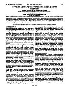
CHAPTER 3 APPROACH: MULTI-ASPECT COMPONENT MODELS As argued in Chapter 1, to be cost-effective, model-based systems engineering must rely on model reuse. In this chapter, we develop a framework for enabling such model reuse by relying on modularity and composition. 3.1 The Structure of MAsCoMs Since current practice in systems design relies mostly on integration of modular components and subsystems, the most common units for reuse are exactly these components or subsystems. It therefore makes sense to organize EAMs by component type also. Whenever a designer decides to use a particular component, he or she will immediately be able to identify all the analysis models that have been previously used to analyze that component or describe its behavior in a larger system. As illustrated in Figure 3.1, the components themselves are organized in a taxonomy so that the user can easily browse from general classes down to very specific instances of components. At each level, the component model is linked to all the relevant EAMs. However, the number of such models could be very large, so that an additional method of organization is desirable. To facilitate the task of selecting and composing analysis models further, we propose to characterize the analysis models based on one or more aspects, as is illustrated conceptually in Figure 3.1. The aspects are orthogonal directions along which a model can be characterized. This is similar to the aspects in Aspect-Oriented Software Development [55], in which modularity is achieved by implementing cross-cutting concerns separately so that they can be woven into a variety
22
FP component
Valve
Relief
Check
Const Displ.
Analysis Model
Model
Model
…
Model
Formalism
Model
DAE
Model
Taxonomy of Aspects
Behavior
Model
…
Var Displ.
Discipline
…
Multi-Aspect Component Model (Set)
Pump
Hydraulic Thermal Algebraic
Model
Taxonomy of Components
Figure 3.1. Multi-aspect component models combine analysis models (EAMs) in a matrix organization linked to taxonomies of components and aspects.
of different software classes. In the context of modeling, rather than the ability to weave models together, what is important is that we can identify which models are compatible with each other so that they can be composed into system-level models.
To be
compatible, models utilized in the composition must characterize the components in a system from a similar perspective, in a compatible mathematical formalism and in the same executable language. By using a formal taxonomy of aspects, the semantics of the individual analysis models are defined in a computer interpretable and searchable fashion. In the remainder of this chapter, the details are provided for how analysis models are organized into MAsCoMs. In addition to discussing taxonomies of components and aspects, it is explained in detail how the analysis models are tightly linked to each other through components at a very fine-grained level.
23
3.2 MAsCoM Model Sets This section is intended to clarify the grouping of models that is contained in a MAsCoM and provide justification for this concept. In our approach, when analysis models are grouped, it is solely by component or subsystem. Each of these analysis models might be thought of as a component model to portray particular aspects of the component, but a MAsCoM is simply the model grouping. MAsCoMs are intended to portray the complete perspective of a component from all angles. This is achieved by grouping enough analysis models about the component to have essentially ‘every angle covered’ (invoking the universal set of aspects). This is a difficult proposition; acquiring a set of models that ‘completes’ a MAsCoM is not likely to happen. The large and extensible list of aspects is such that a complete MAsCoM would require models about the component from every lifecycle phase, discipline, time and space discretization, mathematical formalism, and programming language. A more likely scenario is that most MAsCoMs will combine models about a component from different disciplinary perspectives and from different library sets, which are typically designed for particular lifecycle phases. In this more realistic scenario, some aspects cut across many models in a MAsCoM, while others are sparse and unique to only a handful of models. A guiding use case for MAsCoMs is that a modeler would use MAsCoMs when creating an analysis test case or designing a system model to primarily determine what EAMs are available to analyze a component, and how these models differ. Additional details about a typical MAsCoM use case are shown in Sections 3.4, 3.5, and Chapter 5.
24
3.3 Taxonomies of Components and Aspects The fundamental principles behind MAsCoMs are the relationships between the EAMs, components, and aspects. In this section we present how these elements of modeling with MAsCoMs are organized and viewed. Both components and Aspects are organized in taxonomies, such that these elements do not exist individually, but as parts of their own knowledge structures as well. 3.3.1 A Taxonomy of Components In design, components or subsystems are selected and defined in an iterative fashion. First, a functional architecture is defined after which functions are assigned to components in a physical architecture [44] (or, equivalently working principles and working structures are identified [36]). The focus is initially on the selection of broad classes of components that share the same functionality. For instance, to implement the function of converting electrical to mechanical energy, the broad class of motors could be identified. In subsequent iterations, this broad class of components is gradually refined until a particular component XYZ from company ABC has been identified. At each step along the way, analysis models at different levels of abstraction are used.
As the
definition of the components still under consideration becomes more and more detailed, the corresponding analysis models also need to become more detailed such that the selection can continue to be narrowed down further. To support such successive refinement of classes of components down to very specific individual components, it is meaningful to organize the components in a taxonomy. One branch of the total taxonomy—the branch of hydraulic components—is illustrated in Figure 3.2.
25
Figure 3.2. An example portion of a component taxonomy.
The component taxonomy is based on the E-class classification hierarchy as an initial breakdown of components in the hydraulics domain [12]. Organizing components into a taxonomy has the additional benefit that one can take advantage of the inheritance mechanism to associate analysis models with components efficiently. In the taxonomy, analysis models associated with parents apply also to children. For instance, since an axial piston pump is a type of displacement pump, the models for the general class of displacement pumps (the parent) also apply to axial piston pumps (the child). However, often, more detailed models are available for the children because more detailed knowledge is available about their structure, size, or other design properties. In most cases, components can have complex internal relationships, and are essentially subsystem assemblies. Many times, what one designer considers to be a
26
component, another considers to be an entire system. For example, an engine is a component in an automobile drive-train system, while the engine itself can be a very complex subsystem.
When considering organizing components or subsystems in a
taxonomy, it is important to recognize the relative complexities of the elements being related in the inheritance structure. Simple parent components cannot typically be specialized into complex child components. Thus, in our approach, an engine would not be organized in a taxonomy of engine parts, but instead in a taxonomy of other engine devices with similar functional interfaces and complexity. The reason for this is that it is difficult to create a hierarchical taxonomy that spans both abstraction and decomposition. Through specialization, more details are added to an abstract component; however, from a component perspective, the additional details of a component’s internal structure cannot be separated further in children of the same taxonomy (this would change the functional nature of the parent component). Each of the nodes in the component taxonomy tree corresponds to a model that defines the key characteristics of the component or class of components, as is illustrated later using SysML in Figure 4.2; we call this a structure model. The structure models are parametric—they contain properties identifying key characteristics of the component: sizing properties, key performance parameters, as well as the intended interface of the component (i.e., the locations or ports at which the component is intended to interact with other components in a system [27]). For instance, a pump may be characterized by sizing parameters that include displacement, mass, or maximum pressure rating; by key performance parameters such as cost, efficiency or reliability; and by an intended
27
interface consisting of two fluid ports (suction and discharge) and two mechanical ports (input shaft and housing). The structure models are central to MAsCoMs—they serve as the central entrypoints for accessing all the engineering analysis models associated with the components. The analysis models in turn define how the performance parameters in the structure model relate to the sizing properties. To facilitate maintaining consistency among all these parameters, the analysis models are tied to the structure model at a very finegrained level as is explained further in Section 3.4. In a typical MAsCoM use case, modelers access EAMs in a MAsCoM through the component taxonomy. The advantage of the taxonomy here is twofold: 1) Modelers can determine the EAMs to use by identifying with a level of component detail (abstraction) represented in the component taxonomy, and 2) As a design evolves, modelers can utilize the knowledge in the taxonomy to find analysis models for more specialized components. After identifying the correct component, it is each model’s relationships with the aspects that are used to differentiate the models for selection. For the aspects, we again turn to a taxonomy for organization. 3.3.2 A Taxonomy of Aspects When reusing a model, one needs to recognize which model is needed from among the many models that may be associated with a particular component. To help the designer do this, models are characterized using aspects, the orthogonal dimensions along which models can be characterized. Since there are a large number of potential aspects, it is helpful to organize them also in a taxonomy, as is illustrated in Figure 3.3.
28
Figure 3.3. An example aspect taxonomy.
The taxonomy also emphasizes that the aspects represent independent directions along which a model can be characterized. As a result, a model is typically characterized by
29
multiple aspects simultaneously.
For example, a hydraulic pump model could be
characterized simultaneously by the hydraulic and mechanical engineering disciplines, by the continuous time discretization aspect, by the DAE mathematical formalism, and by the Modelica representation syntax.
A glossary of all aspects used thus far in the
MAsCoM framework is presented in Appendix A. These aspects formally characterize an model and thus succinctly provide the designer or analyst with the basic information needed to select from a set of EAMs that represent a particular component. Additional information about the model can be defined as meta-data that is less structured, such as model documentation, development history, or prior usage scenarios. Based on the aspects, a designer can efficiently search or browse through a model repository to identify the model that is most appropriate for a particular design context. In addition, when composing multiple component models into a system-level model, the aspects provide necessary information to determine compatibility between models. For instance, to be composed, models need to be expressed in compatible mathematical formalisms and levels of discretization—it is not meaningful to combine a high resolution, discrete event simulation model with a low resolution, partial differential equation model. Models that are composed also should be characterized by compatible engineering disciplines. One set of models may describe the hydraulic behavior of a system while another may describe its mechanical structure.
Having formal
representations of these different aspects available is particularly important when considering (partially) automating the composition process.
30
Now that we have described how to initially classify, and potentially select EAMs for reuse from MAsCoMs, we focus on additional relationships between components and models, such that a modeler will also understand how best to use the model. 3.4 Fine-grained Structure-to-Behavior Relationships While the characterization of EAMs using the component and aspect taxonomies reduces the cost of identifying appropriate models for reuse, it does not affect the cost of instantiating these model in a specific design context. One of the goals of MAsCoMs is to facilitate (and maybe automate) this instantiation of analysis models into a systemlevel analysis model. In a variety of engineering disciplines, it is common to describe systems as compositions of components in a schematic diagram. One can interpret such diagrams as compositions of structure models (as defined previously in this section) connected to each other at their ports (intended interface locations). Assume that a system schematic is available in which specific structure models for individual components have been configured into a system by connecting their ports. Is it then possible to instantiate the corresponding analysis models and configure them into a system-level simulation? The additional knowledge necessary to support this context-specific instantiation can be incorporated in MAsCoMs with two additional diagrams: parameter maps and interface maps. Parameter maps bind the parameter values in analysis models to the related parameters in the corresponding component’s structure model. In the context of systems engineering, the values for the parameters need to be related to the properties of the system alternative that is currently being analyzed. Since we have associated the analysis
31
models with components in the component taxonomy, it becomes possible to establish these relationships also in a reusable fashion. How this is accomplished using SysML parametric diagrams is explained in Section 4.4. In addition to parameter maps, MAsCoMs also include interface maps. Interface maps support the configuration of the interfaces of analysis models for individual components into system-level analysis models. Similar to the composition of structure models into a system schematic, analysis models can be configured into networks through well-defined port-based interfaces [37], as is implemented in tools such as SimulinkTM [49], and in languages such as Modelica [32].
Recently, the ability to
compose analysis models has even become feasible for finite element models [5, 48]. In order to configure the analysis models, one needs to define how the ports of the analysis models relate to the ports in the structure models. This is accomplished through interface maps as is further explained in Section 4.3. A final comment related to parameter and interface maps revisits the question of why they are necessary. One could have used other mechanisms for linking analysis models to component-structure models.
For instance, one could have relied on the
inheritance mechanism to associate analysis equations with the properties in a component-structure model. However, that would require that the model equations be expressed using the same property names as used in the component-structure model. Since it is often the case that one analysis model is associated with multiple componentstructure models, and that one component-structure model is associated with multiple analysis models, it would become nearly impossible to develop a reusable model library in which all the property names remain consistent across both analysis and component-
32
structure models. The mechanism of mapping parameters and junctions in a model context provides the needed flexibility to define modular, reusable analysis models independently of the components with which they may be associated in the future. We have highlighted how the MAsCoM approach classifies analysis models for identification and for reuse. Now, we focus on the knowledge required for automated system model composition, and justify the contribution MAsCoMs can make in this area. 3.5 How Can MAsCoMs Support Computer-Automated Composition? In typical design scenarios, an expert user (human) is involved in the following tasks: •
Matching of model context knowledge with analysis context requirements:
The
required characteristics for models needed for specific analyses must be determined and models from a repository that satisfy these requirements must then be identified; •
Composing component models to generate system models:
Models selected to
predict component behavior must be connected to each other to predict the system’s behavior; •
Administering the test case of the analysis to the system model: The system model parameters and boundary conditions must be set for the test case, and the model must be simulated.
Domain experts are also directly involved in the development of meaningful test cases, the interpretation of analysis results, and the direction of redesign. For our purposes here, we focus on the tasks of identifying models and composing models into a functional, declarative system model that can represent a system design in an analysis test case. We refer to these as the ‘composition tasks’. The purpose of this section is to outline what
33
knowledge is used—and thus must obtained from an expert user or computer—to perform the composition tasks.
This knowledge is broken down into two different
classes: (1) Analysis context knowledge and (2) Model context knowledge. (1)
Analysis context knowledge is an input to the composition tasks; it is used to
specify: •
The form or structure of a design concept — e.g., a schematic;
•
The type and depth of analysis that is required;
•
The analysis context details, such as simulation parameters, boundary conditions for the test case, or the desired interfaces at the boundary of the system model.
This analysis context knowledge is not found for reuse in the MAsCoM framework. It will either be specified by expert users (or managers), or it could possibly be derived from existing knowledge from previous design efforts. (2)
Model context knowledge. This type of knowledge is available in MAsCoMs,
and includes the following: •
Model semantics;
•
Model interface definitions, compatibility details, and relationships with component ports;
•
Model parameter definitions and relationships with component attributes.
Assuming that the analysis context knowledge is provided by the systems engineer, then MAsCoMs provide all of the necessary model context knowledge to support automated composition. MAsCoMs provide model semantics by describing model relationships with components and aspects. MAsCoMs define interfaces with interface maps, and
34
express the compatibility of such interfaces by expressing them as interface ports of specific types. Lastly, MAsCoMs define the model parameters with parameter maps. Let us now consider how we can use the model context knowledge provided by MAsCoMs to support a composition of models. Given a design concept that describes a system of interest, we first recognize the components that comprise the system. For each component, we consider its level of abstraction, interface ports and other attributes as specified by its Type, so that we can locate the component in the component taxonomy. Next, given the context of an analysis, a model of the component can be selected from the MAsCoM to support the perspectives of the analysis, which can be represented by aspects from the aspect taxonomy. This involves identifying a match between the analysis context knowledge and the model context knowledge for each model in the MAsCoM (i.e., ensuring that the model represents the aspects required for the analysis). In addition, the attribute values of the design concept component can be mapped to the parameters of the selected behavior model using the knowledge in the parameter map. Finally, we can compose all of the selected models together to form a model for the entire system. Model interface ports are connected with guidance from the interface maps to resemble the design concept structure. For example, in a dynamic behavior composition, the models are connected in a way that closely resembles the same system architecture as defined in a structural model of the design concept. This will be further illustrated in Section 5.1.4. Although we have identified much of the knowledge involved in the composition tasks and how MAsCoMs support these tasks, we acknowledge that we cannot ignore the additional specialized knowledge expert modelers may use when composing models of
35
system analyses.
Removing a human—a domain expert—from design and analysis
activities entirely is difficult. Much of the knowledge experts contribute to systems models is in the form of experience with a tool, a particular model’s behavior, or a fundamental understanding of a model’s equations. It is generally difficult to capture the context in which this expert knowledge is applied. Still, automated composition may provide a good starting model that can then be refined by the system expert. Only for small classes of problems in certain restricted application domains do we expect that model composition can be fully automated. Some of the expert knowledge can be recognized and substituted by standardizing model interface ports. Standardization is useful especially for the integration of analysis models [54]. Analysis models often use standardized interfaces, formalisms, or syntax for compatibility within a particular tool or analysis model library. Model composition can then become a simple case of matching interface ports.
Within the modeling
community, this is currently achieved by standardizing model libraries.
By using
component models from the same library in a composition, compatibility is implied. In summary, some of the knowledge required to formulate an analysis model is external analysis context knowledge. Model context knowledge on the other hand is captured through model organization and can be represented with MAsCoMs. Human modeler knowledge that is built on experience and expertise is difficult to capture, although some of this experience can be captured by using standardized model interfaces in standard model libraries. Even when MAsCoMs do not represent all the necessary knowledge for automated composition, they can partially perform the composition task so that the expert only needs to focus on implementing the necessary model refinements.
36
CHAPTER 4
IMPLEMENTATION OF MASCOMS IN SYSML
To make MAsCoMs useful in the context of systems engineering, all the concepts and relationships have been defined in the Systems Modeling Language (OMG SysMLTM) [51].
Since SysML has been defined specifically to support systems
engineering, it includes modeling constructs that directly support the definition of physical architectures and engineering analyses—the main focus of MAsCoMs. In the next section, some common SysML constructs are explained for the benefit of those who are not familiar with the language. For additional clarification, see the current version of the SysML specification [51]. If you are proficient in SysML, you may skip to Section 4.2. 4.1 Application of SysML Modeling Constructs and Diagrams A sample set of SysML constructs and diagrams is illustrated in Figure 4.1 and is further explained in this section. The diagrams shown were created in MagicDraw UMLTM [28], a SysML modeling tool. The primary modeling construct in SysML is the block. A block can represent anything, whether tangible or intangible, that describes a system. For instance, a block could model a system, process, function, or context. In this work, the use of blocks includes the modeling of component structure, aspects, engineering analysis models, and interface junctions. Blocks are declared in Block Definition Diagrams (BDD), as can be seen at the top left in Figure 4.1. A BDD is used to define block features and the relationships between blocks or other SysML constructs and is thus the equivalent of a class diagram in UML [9].
37
Figure 4.1. SysML diagrams and representative constructs in MagicDraw.
In the figure, a block ‘BlockA’ has two block properties. One, named ‘block property’ is of type ‘Valuetype’. A second property, ‘Mass’, is of type ‘Mass’ in units of kilograms. Neither of these properties shown here is quantified. Two composition relationships exist between BlockA and its constituents, BlockC and BlockD.
This
means that BlockA exists as a set of blocks C and D, although the set (BlockA) can also own additional properties itself. Finally, in the BDD in Figure 4.1, BlockA is generalized by BlockB, meaning that it inherits its properties from BlockB. This is shown by the white arrow, or generalization relationship in SysML. A variety of other relationships that are built upon the definition of blocks are included in Internal Block Diagrams (IBD), as shown at the bottom left in Figure 4.1. In the figure, a block named ‘BlockA’ has a port ‘portA’ that is of a specific stereotype ‘flowport’. This port has an outgoing flow.direction specified, and the flow moves to an
38
incoming flow port of a block named ‘BlockB’. BlockB is used in this diagram under the specific usage name ‘UsageName’. To express mathematical constraints, a different type of block, called a constraint block, is used.
Constraint blocks are used to relate parameters through constraints
expressed in an equation-based mathematical formalism or in a specific imperative programming language. Parametric Diagrams (PAR), top right in Figure 4.1, allow one to express constraints between block properties via binding connectors. For example, in the figure, the ‘Mass’ attribute of ‘BlockA’ is related to the ‘Mass’ parameter of ‘ModelA.’ If this were a simple equality, a constraint (and associated constraint block) would not be needed; however, in this case, a change of units requires these block properties to be related via an equation.
Lastly, constraint properties are used in
constraint blocks to represent specific parameters in the constraint equation, or they can exist individually in parametric diagrams, such as ‘GPext’ in Figure 4.4. In this case, ‘GPext’ is represented as a default value for a model parameter that is not equal to a typical component attribute. Package diagrams (PKG), shown at the bottom right in Figure 4.1, are used to illustrate the organizational structure of a SysML model by using a containment relationship to contain parts of the model in different folders, or packages. This is similar to the organization of folders in a file system. Packages contain entities such as blocks, diagrams, and other packages. Between SysML entities, two other relationships can be modeled:
39
•
Dependency: This is used to express the reliance of one entity upon another (see the bottom right in Figure 4.1). This relationship is the most general relationship and has a weak syntax that can be strengthened (clarified) via additional stereotypes.
•
Stereotypes:
These provide a way to specialize SysML constructs.
Through
stereotypes, typical SysML constructs can have their semantics restricted to meet the needs of a design model. Examples of stereotypes include blocks and constraint blocks, which are restrictions of the UML construct class [51]. In MAsCoMs, the dependency relationship is stereotyped as «refine», which conveys the new meaning that one entity is a refinement of another. While these are not all the constructs available in SysML, they are a good starting set for modeling MAsCoMs. 4.2 Modeling Taxonomies of Components and Aspects Both the component and aspect taxonomies are modeled in SysML using the generalization relationship, as illustrated in Figure 4.2. A generalization signifies that all the properties of the parent block—the block pointed to by the white arrow—are inherited by the child block. Defining the taxonomy of components in this fashion simplifies the definition of additional components because most of their properties are likely to be inherited from existing component definitions.
As is illustrated for a
commercial off-the-shelf pump, Vendor_OTS_Pump, SysML also allows one to further restrict the values of inherited properties.
Finally, besides certain key sizing and
performance properties, the blocks also define the intended interface of the component, e.g., the suction and discharge ports of the pump.
40
Figure 4.2. This branch of the component taxonomy shows the hierarchy of structuremodels that define the component interfaces and key characteristics.
An important additional benefit of using generalization relationships is that all the engineering-analysis models associated with a parent also are associated with its children. For instance, when defining an additional pump from a specific vendor, there is no need to associate explicitly an entire set of analysis models with this new structure model, because the specific pump can simply be a specialization of an existing pump model and, as such, inherit all the analysis models associated with all of its parents. To help the user browse through the set of component models, the blocks are organized in packages, as is illustrated in Figure 4.3. This has the additional advantage that name clashes can be easily avoided because they only need to be unique within the
41
namespace of the local package. Globally, name clashes are avoided by using fully qualified names (e.g., Component.HydraulicComponent.Pump.FixedDisplacementPump.VendorOTSPump rather than VendorOTSPump). Similar to components, aspects are organized into packages, and the generalization relationship is used to structure the aspects hierarchically. Typically, only leaves of the aspect taxonomy are used to classify a model, since the intent of MAsCoMs is to enable reuse by capturing knowledge about the model in as much detail as possible. However, when specifying the context of analyses, upper-level aspect classifiers are often useful to specify a general class of model that would be applicable. A glossary of all the aspects used thus far in the MAsCoMs is presented in Appendix A. 4.3 Model Context Diagrams To describe how a specific analysis model relates to a component structure model, a Model Context is defined, as illustrated in Figure 4.3. For each matching pair of specific analysis model and component structure, a different Model Context is needed. The idea of mapping analysis models to structure models in a specific context was developed previously by Peak et al. [40]. They introduced Context Based Analysis Models (CBAM) to bind the parameters of an analysis model to values in a structural model in the context of a specific analysis. If the analysis model is defined to be sufficiently general, it can be reused in multiple contexts. For this work, it is recognized that, for a particular component, such bindings between analysis models and structure models often remain the same irrespective of how the component is used within a larger system. It therefore makes sense to establish these bindings at the component level so that the mapping becomes reusable.
42
Figure 4.3. Model context BDD of the ConPump model from the Modelica HyLib library [33].
To relate an analysis model to the elements in the component and aspect taxonomies, the SysML relationship «refine» is used.
For instance, the «refine»
relationships in Figure 4.3 reflect that the ConPump analysis model refines the description of the Fixed_Displacement_Pump component and that it refines a generic hydraulic behavior model, a mechanical rotational model, etc. Note that, as with most SysML diagrams, only the relevant information is shown. One must keep in mind that the component is related to many other components in the component taxonomy and that the aspects are also just references to their definitions in the aspect taxonomy.
43
4.4 Parameter Maps Now that since the analysis model is linked to its aspects and to a corresponding component, the detailed parameters of the model can also be mapped in a reusable fashion. As shown in Figure 4.4, the parameters of an analysis model can be bound to their corresponding properties in the component-structure model. The binding connector has the semantics of a noncausal equality. If necessary, additional constraint blocks can be used to bind properties that are related but not exactly equal.
For instance, the
displacement property of the ConPump model is related to the displacement property of the Fixed_Displacement_Pump component through a constraint block that imposes the appropriate unit conversion. In addition to unit conversions, a similar constraint block could be used to map related properties to each other, such as radius to diameter or radius to surface area.
Figure 4.4. A parameter map for a displacement pump.
44
To support composition of port-based analysis models [37], the Model Context in Figure 4.3 also includes a detailed interface mapping. By formally linking interface junctions in the analysis model (e.g., p:FluidJunction) to the corresponding ports in the structural model (e.g., discharge:FluidPort), the component-level analysis models can be composed into a system-level analysis model based on the composition of componentstructure models in a system configuration model. Now that we have reviewed the implementation of MAsCoM knowledge in SysML diagrams, we step back to discuss a few best practices of the implementation of a reusable MAsCoM library within MagicDraw UMLTM [28], the SysML modeling tool used for this work. 4.5 MAsCoM Library Organization—Best Practices Large-scale, complex design efforts can likely have their value increased through the use of formal modeling in MBSE and the MAsCoM approach. Consider an example scenario where a design effort is captured formally in an information model via SysML. Typical design information based on MBSE is captured for storage, maintenance, and interfacing to other design tools. When organizing the design information, MAsCoMs can be easily referenced to link analysis models and components with analysis test cases. Much experience linking components, models, and analyses has been gained through working with MAsCoMs in several design examples, including those in Chapter 5. In this experience, a general approach that has been found viable separates design information, a MAsCoM library, and a library of analysis models. This approach is also supported by the modeling and execution of analyses through graph transformations by Johnson [22]. One has to keep in mind that MAsCoMs, while information models
45
themselves, do not actually contain analysis models. Instead, MAsCoMs refer to analysis models that are stored in their native model libraries. Figure 4.5 highlights the general package organization of a MAsCoM library used in a design effort. The MAsCoM library is initially divided into packages containing the component and aspect taxonomies. A third package contains the junction definitions of standard interfaces used by MAsCoM model context definitions, interface maps, and junction maps. Finally, a fourth package contains the MAsCoMs themselves. In the model library, analysis models are described in terms of SysML constructs, organized in a model library package and subdivided by their originating tools and toolboxes. The interfaces of models are captured and stored as blocks in the MAsCoM library interfaces package, so that the interface can be captured in a block property definition in the block used to represent the model. Finally, once interface junctions for each model interface have been established, these junctions can be used in an interface mapping in the model context diagram.
46
Figure 4.5. Package organization of a MAsCoM library as used in a design effort.
Each MAsCoM is represented as a block in the library. This block is used to hold all relevant information and knowledge about the MAsCoM. This includes diagrams
47
such as model context diagrams with interface maps and parameter maps. Also included are the relationships established in each diagram, the usages of entities from the component taxonomy, aspect taxonomy, or interface package in a diagram, and any other entities or relationships created specifically for a diagram of the MAsCoM. In summary, by defining such diagrams for a large number of analysis models, a library of formal, reusable models (MAsCoMs) can be defined to capture the knowledge about analysis models in a particular domain of interest. These libraries combined with existing SysML constructs for requirements, test-cases, functional allocations, system behavior, and use-cases provide the systems engineer with a complete language and vocabulary for efficiently and effectively defining and evaluating system alternatives in a formal fashion. We now illustrate the use of the MAsCoM approach and implementation in three design examples in an attempt to validate their contribution of value to design problems.
48
CHAPTER 5
USING MASCOMS IN DESIGN EXAMPLES
In this chapter, three fluid-power examples are used to show the value and details of using MAsCoMs. The first example, the hydraulic system of a log splitter, illustrates how MAsCoMs can be used in the design process. A second example consists of a hydraulic system of a scissor lift in which the value of component model reuse is demonstrated. Lastly, we present the capture of a complex component model into a MAsCoM of a component used in the hydraulic system of an excavator. For these examples, we assume that the designer has previously defined a particular design problem by modeling the system objectives, requirements and functional decomposition in a SysML design model. The designer then needs to consider which measures of effectiveness (MOEs) can best be used to predict the extent to which certain objectives are satisfied. This is where analysis models play a role. Analyses must be specified such that the MOEs can be predicted based on an analysis model. 5.1 Example A: Log Splitter Although a log splitter is relatively simple, it is representative for a broad class of hydraulic devices. In this example, we focus on a key aspect of component model reuse—the reuse of modular analysis models through composition into a desired system model. Through composition, system models for any design concept can be created quickly and cheaply from their modular parts. Furthermore, these models can easily be reconfigured to further evaluate such designs. As illustrated in a schematic in Figure 5.1, the hydraulic circuit of a typical log splitter contains a flow device (shaft-driven pump), a flow control device (servo valve), a
49
hydraulic actuation device (double-acting cylinder), a filter, tank, and hydraulic lines. Larger hydraulic systems can be thought of as variants of this circuit with additional actuators or more complex control logic.
Figure 5.1. A simplified schematic of a design concept for a log splitter.
While the schematic of the hydraulic system represents the design concept, it does not allow for a seamless integration with other design knowledge in the context of MBSE and MAsCoMs.
To integrate the design concept with a formal analysis, we must
formalize its schematic in SysML. 5.1.1 Defining System Composition and Function from a Schematic To formalize a design concept via a schematic in SysML, one must consider the types of information that are contained in a typical engineering schematic.
This
information includes component types and ports, as identified by ISO symbol representations, as well as the connections between the components’ ports. In SysML, the log splitter hydraulic system can be represented as a block, which in turn represents a system consisting of the composition of several component blocks. The details of the assembly of component blocks that comprise the system block can be modeled through the system block’s IBD, as shown for the log splitter in Figure 5.2. In
50
the IBD, the structural ports of the structure model of each component are shown and connected to represent the same information as would be found in the typical engineering schematic.
Figure 5.2. System structure-model IBD for the log splitter design concept.
5.1.2 Defining an Analysis Context to Test System Performance in a Discipline Once a concept is captured in the design model, it can be tested. This test is a specific operation that the concept undergoes in a particular environment. The test is designed to measure system behavior and performance from the perspective of a
51
particular stakeholder. Rather than performing the test on a physical system, it is often less expensive to use a virtual, simulated system. In this way, the system behavior is predicted rather than measured, and many more quantities than in physical experiments can be assessed. The analyst may characterize the context of an analysis by specifying which measures of effectiveness (MOEs) need to be predicted and by defining the particular aspects that need to be considered in the system-level model of the concept. A complete analysis context will frame the test case used to investigate the design concept and specify the type of model used to represent the concept in such a test case. This is an important point; while a design concept can be physically instrumented and tested from any possible perspective, an analysis model is typically only usable in testing the concept from a very specific perspective. The simulation that exercises the model to perform the analysis can then be used in a SysML test-case to verify whether the requirement for the given MOE is satisfied. An analysis context for a system concept can be outlined in terms of simulation parameters [22], aspects, and through a relationship to a test case that stores additional information if applicable.
Test case information may include simulation boundary
conditions, links to requirements and MOEs, and test processes and procedures. An example analysis context for a log splitter hydraulic system is illustrated in Figure 5.3. Blocks are used to capture the simulation of the model used to support the analysis, the system model that will be exercised in the analysis, and a test case if applicable. Aspects from the aspect taxonomy are referenced to specify the general type of the set of models used to compose the system model.
52
Figure 5.3. Characterization of the context of a system-level analysis for the log splitter design problem. A log splitter hydraulic simulation (LSHS) predicts the efficiency MOE.
Notice that in Figure 5.3, the block for the Hydraulic System model is still empty. This represents the fact that an analysis can be specified without yet having a detailed model to support it. In the next section (5.1.3), the process for filling in this block is explained. 5.1.3 Component Model Selection The creation of this system-level analysis model starts by defining the particular system architecture that will be analyzed, as illustrated in Figure 5.1 and formalized in
53
SysML in Figure 5.2. The system architecture is a composition of component-structure models connected by their ports.
Depending on how far the design process has
progressed, these component-structure models could still be very abstract (i.e., close to the root of the component taxonomy) or very specific (e.g., a specific pump from a specific manufacturer).
Throughout the design process, these component-structure
models are likely to be refined into more and more specific models from the component taxonomy. If a particular component-structure is not yet available in the component taxonomy, then the user may need to create a new model. Such a new model can be defined most easily by first determining where in the component taxonomy it would fit and by then extending the appropriate parent models through specialization relationships. In this way, all the analysis models of the parents are also automatically associated with the new child. If additional analysis models are required then they can be added by defining additional model context diagrams. Note that such additional models should be defined in a local user-model rather than added to the MAsCoMs library right away; since the library is likely to be (re-)used by many different users, it should be kept under strict version control, and models should only be added to the library after extensive verification and validation. Once the system architecture has been defined, one can use the model context diagrams in the MAsCoMs library to provide the necessary information for identifying the appropriate analysis models.
Although there are potentially a large number of
analysis models associated with each component in the taxonomy, the aspects that characterize the models allow the designer to home in on the few that are applicable in
54
the given context. To be applicable, a model needs to include the same aspects as have been defined for the system-level model analysis context (as in Figure 5.3). The aspects also help the designer to determine whether the component models are compatible with each other (e.g., from the same native model library). Once the appropriate models have been determined, the specific values of the component properties can be instantiated through the use of parameter maps. Alternatively, the task of instantiating specific parameter values can be postponed if the system model will be used in a more general context and will therefore be stored for reuse. At this point, the set of component models needs to be connected to form a system model. 5.1.4 System Model Composition The final step towards a complete system-level model is to integrate the analysis models of the individual components with each other. As mentioned in Section 3.5, this composition requires additional knowledge beyond what is currently available in the MAsCoM library. This knowledge is algorithmic in nature—it cannot be captured in a static diagram (i.e., a schematic), but instead requires the specification of how the diagrams need to be manipulated or transformed. In the current implementation, this composition is left to the user.
However, in the future, we plan to automate this
composition process through the use of graph transformations as has already been demonstrated for SysML diagrams by Johnson et al. [22]. The composition process is illustrated for a portion of the log splitter hydraulic system model, the power subsystem, shown in Figure 5.4. Although the topology of the analysis model is very similar to the topology of the system-structure model in Figure 5.2, it is not a one-to-one mapping. As is explained in more detail in [23], the connection
55
of energy-based ports, such as a FluidJunction, requires the inclusion of a model representing the equivalent of Kirchhoff’s voltage and current laws.
Figure 5.4. Dynamic model for a portion of the log splitter example (shaded boxes represent external interface ports requiring further connections).
To connect the interfaces of the models in this log splitter power subsystem, ‘FluidNodes’ are used to connect the models’ ‘FluidJunctions’.
The ‘fluidnode’
constraints are used to apply the equivalent of Kirchhoff’s laws by constraining the interface parameters of the junctions. Each fluidnode in this example joins two fluid
56
junctions based on SI units, except for the node joining the filter to a line connecting to the tank. The orifice model used as a filter in this example uses English units (denoted by FluidJunction.E). The fluidnodes are also used to convert the interfaces of the orifice model to SI units. 5.1.5 Composition of Reliability Models In systems engineering, conflicting objectives often require tradeoffs between measures of effectiveness in multiple disciplines.
For instance, the discipline of
reliability engineering may be tightly coupled to system dynamics or cost considerations. In this section, we demonstrate the capability to represent and reuse analysis models from the reliability discipline through MAsCoMs. Reliability models do not match the topology of a system structure model since they represent a coupling of functions mapped together to perform a system level function. Essentially, reliability models are not connected in the same way that the physical components are connected as shown in an engineering schematic. To compose reliability models, the relationships between component functions and critical system functions must be determined so that a meaningful reliability composition will be achieved. One way to achieve this mapping cost effectively is to use graph transformation algorithms to transform the system structure into a form that can be used by reliability modeling methods. Although the implementation of such transformations is beyond the scope of this current thesis, we explore how to perform such compositions manually for the case of probabilistic risk assessment, or PRA [25]. Within PRA, fault trees are a common method for predicting the probability of failure. Just as for other perspectives, fault trees
57
can be composed with reusable component models and interfaces.
Since reliability
models are not based on energy exchange through ports, their topology does not match the topology of the system-structure model.
Instead, the composition of reliability
models in a PRA analysis involves tying all component analysis models together via logical nodes, as is shown in Figure 5.5.
Note that the model in Figure 5.5 has
parameters for quantifying the numbers of several component ports, shown in an interface mapping. We can combine this model into a fault tree to represent the control subsystem of a hydraulic circuit, shown in Figure 5.6.
Figure 5.5. Model context diagram for the reliability model of a hydraulic servo valve.
58
When reliability models are composed, they are typically linked together into chains to represent the dependency of one component’s operation on other components. Essentially, this means that one component’s probability of failure is dependent upon both its own reliability in addition to the reliability of other components it depends upon. Although reliability itself is defined as the probability of success (i.e., 1 – probability of failure), the fault trees shown in this work capture the probability of failure and trace the propagation of this probability from the component level to the system level.
Figure 5.6. Reliability model for the log splitter.
To consider a reliability perspective using models from MAsCoMs, we formally capture the fault tree model of a pressure-compensated, load-sensing hydraulic system. In Figure 5.6, a composition is illustrated for a single level of a fault tree. There are a few important distinctions to note in this fault tree reliability composition. First, the models shown in the figure are represented as constraint blocks, an alternate representation of a model in SysML. Generally, this is useful for simple models whose
59
equations can be made visible via constraints, and properties shown as constraint properties. Complex models (with many more equations) can still be represented as blocks with parameters as part properties. A second distinction is the choice of what to show in a diagram. Since reliability model compositions can become quite large, it makes sense to break up the models into a series of diagrams. Due to the hierarchical nature of fault tree diagrams, parametric diagrams are a logical choice for implementation.
Parametric diagrams can be
hierarchically structured, similar to portions of a fault tree. SysML parametrics allows for a convenient nesting of parametric relationships to enable the hierarchical structuring and reuse of the relationships. A possible disadvantages of the nested structuring of PRA diagrams is that the nesting can leave many component model parameters hidden deep within the system model; this makes it difficult for a modeler to assign values to these parameters. Also, the logical failure path of a system reliability model is more difficult to visualize when captured in nested diagrams; although, the diagrams are traceable and the path can be deduced. Since system structure diagrams (schematics) do not reflect the reliability structure either, an alternate form for the system composition is necessary (without nesting) to improve the comprehension and communication. Just as nodes are used for combining junctions in model compositions of dynamic behavior, nodes of reliability models are used to represent the logical constructs of fault trees and to join component models together. Like dynamic model nodes, reliability modeling constructs such as logical nodes for fault trees can be captured formally and stored within a MAsCoM library’s interfaces package.
60
5.1.6 Composition of Accounting-based Models An additional common perspective of modeling is that of a simple accountingbased model composition. The purpose of such compositions is to evaluate a shared parametric property or attribute among multiple components and determine how this property at the component level is related to the property at the system level. The purpose of this section is to address this modeling perspective as it relates to system compositions of cost models. Consider the MAsCoM of a valve component that contains the valve reliability model seen in Section 5.1.5. Assume that this MAsCoM also contains a cost model of the same valve. The model context for the cost model is shown in Figure 5.7. This cost model is characterized by similar aspects as the reliability model in Figure 5.5, yet is distinguished by an ‘Economics.Cost’ discipline aspect and is built as a Microsoft Excel file. The parameter map for this cost model is shown in Figure 5.8. Note that the model inputs of ports, ways, and positions are tied to constraint properties in the parameter map. Thus, the reuse of this valve model in the valve MAsCoM is specific to this model’s context that is related to a 4 port, 3 way, 2 position servo valve.
61
Figure 5.7. Model context diagram for the cost model of a hydraulic servo valve.
When composing an accounting-based system model of component models, it is important to ensure all models share the following: •
The property to be composed (i.e., property type with units);
•
Quantification of the property (with our without uncertainty);
•
Quantity of matching items containing this property (multiplicity for identical components).
62
Figure 5.8. Parameter map diagram for the cost model of a hydraulic servo valve.
In accounting-based compositions, the diagram view of the composition can often be much simpler than the system structural view itself.
This is because duplicate
components only need to be represented once, unless they are not strictly identical. In this way, accounting-based compositions can closely resemble engineering bills of materials (EBOMs), allowing for an easy transformation between such compositions and EBOMs. An example of a cost composition for the control subsystem of the log splitter is presented in Figure 5.9, where a valve model characterized in Figure 5.7 and Figure 5.8 is composed with a hydraulic line model. In this composition, a single valve and four hydraulic lines are composed into a control subsystem. A constraint block containing an addition constraint is used to tie together a weighted sum equation with each model’s cost
63
and quantity to generate the total subsystem cost. The total subsystem cost is the output at the top of the parametric diagram, allowing it to be reused as a nested model (constraint) in other parametric cost model compositions.
Figure 5.9. Control subsystem cost model composition for the log splitter hydraulic system.
The composition of simple accounting-based models requires little knowledge about system architecture—solely which components are involved, their models, and their attribute data. Thus, this is a good starting point for automated compositions, where graph transformations can be applied to a composition that lacks form, and only the rules of property matching and adding are necessary. While it is beneficial to use MAsCoMs once to create a system design model, the focus of this work is to provide an effective representation of analysis models that have good opportunity for reuse. In the lifecycle of a MAsCoM, which incurs costs of formal modeling and savings from reuse, value can only be added to design projects through multiple reuses. Thus, we now focus on an example of analysis model reuse in the fluidpower domain by analyzing the hydraulic system of a scissor lift.
64
5.2 An Example of MAsCoM Reuse—Hydraulic Scissor Lift The main reason for modeling the relationships between component models in MAsCoMs is to promote reuse. One opportunity for reuse exists within the context of a design problem whenever two system alternatives are considered that share similar components or subsystems—a very common occurrence. Additionally, reuse is often possible when solving different design problems but still within the same application domain. For instance, consider the design of the hydraulic system of a scissor lift. Although a scissor lift is quite different from a log splitter in principle, it does share the need for compact, large-force actuation for which hydraulic components are well-suited. The schematic for a possible hydraulic system alternative for a scissor lift is illustrated in Figure 5.10; the corresponding system structure-model is shown in Figure 5.11.
Figure 5.10. A simplified schematic for a scissor lift.
This design shares the same power-subsystem as the log splitter shown in Figure 5.4, yet uses a simpler 3-port control valve and a single-acting hydraulic cylinder.
In fact,
between the two concepts, only two analysis models are not reusable—models for a control valve and an actuator.
65
Figure 5.11. System structure-model for the scissor lift.
To see the differences between the actuation portion of the hydraulic circuit, one can visually compare both versions of the model compositions for this part of the circuit in Figure 5.12 and Figure 5.13.
66
Figure 5.12. Dynamic behavior model for the actuation subsystem portion of the log splitter example.
Figure 5.13. Dynamic behavior model for the actuation subsystem portion of the scissor lift example.
The comparison between the required analysis models for the log splitter and scissor lift demonstrates the value of MAsCoMs for identifying and reusing components
67
and analysis models within the same application domain. In this case, the domain of reuse is hydraulic fluid power. However, the reuse of analysis models between these two systems is also subject to some practical considerations.
First, the analysis models used to investigate the
behavior for either system exist at a particular level of abstraction. Thus, for these two design concepts to share the same analysis models, the contexts of the analyses must specify a similar level of abstraction. A second consideration for component model reuse is that of the sizes of the components must be sufficiently similar so that the same models can be used. For example, consider the case in which the size of the pump component used in the log splitter is much smaller than the pump used in the scissor lift. The size is captured in the sizing parameters of the pump structural model and instantiated in the parameters of the pump analysis model. To share analysis models, the size of the sizing parameters for both pumps must be within a range of values within which the analysis model’s behavior has been validated. To avoid such problems, acceptable parameter ranges can be specified for model parameters in model context BDDs. Since a MAsCoM structural model is related to an entire set of analysis models that refine the structure model, once such a set of models is identified, all corresponding analysis models for the structure model (i.e., the pump) are identified for reuse. Ideally, as long as each analysis model in a particular MAsCoM is specified in enough detail with constructs from the MAsCoM framework, one should theoretically be able to determine the most appropriate model to fulfill a case for reuse from the MAsCoM.
68
In the next example, we view MAsCoMs from the perspective of a model library administrator. In the example, a component model for a complex hydraulic component in an excavator hydraulic system is classified for reuse as a MAsCoM. 5.3 Classifying a Model for Reuse as a MAsCoM—Power Unit Component of a Hydraulic Excavator At this point, we have demonstrated how MAsCoMs are used to provide value in design examples. An important perspective of MAsCoMs is the consideration of the costs of formality for the classification of models that exist in a vendor library or that are developed separately. In this example, we compare the costs and benefits of two methods that can be used to capture a complex component model.
We consider a complex
component model to be a model that contains an internal structure of low-level components, such as a subsystem. Such models contain knowledge about how the lowlevel components are connected structurally, as well as how the low-level component attributes are related to the complex component attributes. In this example, to capture a complex component, the following methods are compared: •
Basic Approach:
Capture the component model and express it as a traditional
MAsCoM. This involves constructing a model context diagram, interface map, and parameter map. •
Minimalist Approach: If the low-level components of the complex component model are already captured as MAsCoMs, then use additional diagrams to represent the missing knowledge (i.e., component connections and attribute mappings). Just as model libraries often build upon their own low-level models, one can build upon low-
69
level component MAsCoMs to capture the knowledge of a complex component MAsCoM. The term ‘minimalist’ is used to reflect the minimal amount of effort applied and costs incurred in representing the model for reuse—we take advantage of as much existing formal knowledge as possible. The context of this task is centered on a complex component that is part of a system model of the hydraulic system of an excavator. The component and system models were developed as part of a custom library of hydraulic models coded in Modelica [38]. A graphical illustration of the excavator hydraulic system model in Dymola [11] is shown in Figure 5.14. In this model, we would like to capture a complex component called a Power Unit (lower center in figure) for reuse as a MAsCoM. This is desirable because it was found that this model has a high likelihood of reuse.
70
Figure 5.14. Excavator hydraulic system model from the FluidPower library [38].
Since the power unit is a subsystem model built upon other existing library models, care must be taken in its representation for reuse. A graphical illustration of the power unit is shown in Figure 5.15. Note the use of 5 component models and two manifolds that comprise the power unit model.
71
Figure 5.15. Power unit model from the FluidPower library [38].
5.3.1 Basic Approach: Capturing the Power Unit as a MAsCoM This approach follows the basic use case of a model repository administrator who is characterizing the power unit model according to the MAsCoM framework. This use case includes investigating the power unit’s native library documentation, the model parameters, the component interface ports, and any other model semantics.
After
developing an understanding of the model, the corresponding constructs in the MAsCoM framework are selected to represent the power unit model. The power unit is captured in a MAsCoM model context diagram shown in Figure 5.16.
72
Figure 5.16. A model context diagram of the excavator power unit model.
The interface map is also shown in the figure, relating the interface of the power unit to the component structure model ports.
Generally, a parameter map would also be
included to complete the classification of the power unit as a MAsCoM. However, in this case, the power unit model does not have many parameters that map to component attributes, so the parameter map diagram is not shown. disadvantages of this approach are discussed in Section 5.3.3.
73
The advantages and
5.3.2 Minimalist Approach: Capturing the Power Unit as a MAsCoM by reusing MAsCoM Knowledge from Low-level Components In commercial model libraries, often more complex models are built upon lowlevel models from the library to increase complexity and functionality. In such libraries, modelers can typically use a low-level model in composition, or they can use a more complex model, regardless of the low-level models it is built upon. This is the case for the power unit model. We desire to capture a complex model, yet MAsCoM diagrams that capture low-level models of the power unit are already available. Since the power unit is a composition of the models described by existing MAsCoMs, we can already understand the definitions of the parameters of the power unit through the parameters maps of the low-level component models. We can also interpret the semantics of the power unit through the aspects used to describe its low-level models. In addition to the details in the low-level component MAsCoMs, in this approach we can add the following details about the power unit to represent it to a modeler: •
The architecture of connections between the low-level components;
•
The mapping that exists between the attributes of the low-level structure models and the power unit structure model. The architecture between low-level components can be captured in SysML in an
IBD of the structure models, illustrated in Figure 5.17. Since the existing MAsCoMs describe the interfaces of the low-level components in interface maps, the only details that are necessary are the connections between component ports. The structural ports of the power unit component are represented as part properties in the left side of the
74
diagram. These ports are connected to the ports of the low-level component structures to represent the power unit architecture.
Figure 5.17. Architecture of power unit from low-level component structure-models.
While the architecture of the power unit defines how it is composed from lowlevel components, we also must represent how the attributes of the power unit component map to the low-level component attributes. For this, a component attribute map is defined; it describes how the low-level component attributes relate to those of the complex component. A component attribute map diagram for the power unit is illustrated in a PAR in Figure 5.18.
75
Figure 5.18. Component attribute map for the power unit.
The attributes of the power unit component are shown as SysML part properties in the power unit block on the left in the attribute map. These properties are related to the attributes of the low-level component structure-models via parametric relationships. Two design constraints are also illustrated in the figure. The first constraint, ‘designconst1’, represents the fact that the total system pressure cannot exceed the maximum allowable
76
pressure of the components or the relief valve pressure (this ensures the correct specification of maximum system pressure). ‘Designconst2’ represents the fact that the volume of the accumulator cannot be greater than the volume of the tank (this prevents the tank from fully emptying of fluid). The MAsCoM of the power unit only needs to contain the diagrams in Figure 5.17 and Figure 5.18 to be complete, since it also references the diagrams of the MAsCoMs of the low-level components in the MAsCoM library. To retrieve the power unit model for reuse in a composition, it could be potentially composed from the lowlevel component models with a graph transformation algorithm. This could be very efficient and provide the flexibility of reconfiguring the power unit model in its component structure IBD or component relationship map if a variation is required for reuse. Alternatively, the complete (already composed) power unit model could be stored for reuse and still be represented with this approach as opposed to the representation with the basic approach in Section 5.3.1. 5.3.3 Evaluation of Approaches for Capturing the Power Unit as a MAsCoM There are advantages and disadvantages for using the basic and minimalist approaches in capturing the power unit. Specifically, the benefits and costs of using the two approaches need to be considered. In the basic approach, all of the knowledge required to use the power unit can be found in the diagrams of the power unit contained in its MAsCoM. In some cases, a model is desired to capture a complex component abstractly, without every detail. The basic approach provides the simple representation of a power unit model that is abstract and can be used to predict general behavior about the power unit component.
77
In the minimalist approach, the power unit model is represented for reuse, albeit in a fashion that uses more diagrams in total and that is more difficult to interpret than with the basic MAsCoM diagrams. The advantage of the additional diagrams—from low-level component MAsCoMs—is that many additional details of the low-level models themselves are available to a user to inspect upon searching for a desired power unit model. Hence, even though it is called a minimalist approach, it actually provides more detail about the model to the user. This approach also provides the ability to specify through additional diagrams (i.e., the structural IBD and component attribute map) and create (potentially through graph transformations) any configuration of the low-level component models into a variation of the power unit model. This is similar to the specification of a system model with an analysis context, except that in the minimalist case the component models are preselected; the specific MAsCoMs are specified by name through the component attribute map and structure IBD. Finally, with the ability to recompose the power unit model from a formal characterization in MAsCoM diagrams, a potential extension of the minimalist approach is to specify any model formally as a component or a system from existing MAsCoMs. The model could be quickly composed through a transformation upon its need for retrieval from the MAsCoM library. If the costs of a graph transformation algorithm are ignored for the time being, the minimalist approach should be less costly than the basic approach, since less new knowledge needs to be formally modeled in SysML. Although the power unit can be captured in the basic approach as a typical component model in a MAsCoM, such as shown in Figure 5.16, this approach does not
78
take advantage of the knowledge available in the MAsCoM diagrams of the low-level components. In a sense, this basic approach can be synonymous with “reinventing the wheel”, a practice that incurs unnecessary costs and that should therefore be avoided. The basic MAsCoM model of the power unit could be easily reused, but many of the details of the internal structure of the power unit would be abstracted away. Such details would be desirable for modelers who wish to know the architecture or assumptions that lie within the power unit model. If some of these details are already captured in the MAsCoM diagrams representing the low-level component models in the FluidPower library, why not represent these details to modelers selecting the power unit for reuse? Unless the amount of detail is overwhelming, it would be best to have the information available when making a decision to use the power unit model. Also, a detriment to the basic approach is that it characterizes a complex model in a static structural configuration. Although such a model is still reusable by instantiating different parameter values for component attributes, complex models are typically less likely to be reusable than simple low-level component models. Thus, the basic approach risks the expense of creating a redundant model characterization if the model does not have a large opportunity for reuse. On the other hand, the minimalist approach provides the opportunity for a more reusable model since it is easily reconfigurable. Yet the approach carries with it the additional complexity of knowledge being represented among more diagrams. Also, the minimalist approach carries the ambiguity of costs and risks associated with the necessity of a graph transformation algorithm that is not currently available to compose the power unit model.
Additional costs occur when using the power unit model in a new
79
configuration. Each new configuration must be specified in formal diagrams, which incurs costs of formal modeling to create the diagrams. However, the additional costs may still be smaller than what are necessary to develop and capture new structurally static configurations of a power unit model. 5.3.4 Composition of the Power Unit from Multiple Perspectives For each stakeholder perspective that is required to analyze the power unit, a unique model composition results. In this section, we present compositions of the power unit’s lower-level components to represent the perspectives of dynamic behavior, reliability, cost and mass. The ability to represent these perspectives varies based on the approach used to capture the power unit. The power unit model described in the each approach in Section 5.3 is a dynamic behavior model. A different model is necessary to represent the power unit component from a different perspective. In the basic approach, this requires different model context and parameter map diagrams for the different models, though they are contained in the same MAsCoM. In the minimalist approach, the perspective of the power unit model is limited by the perspective presented by the low-level component models and the structure of the model defined in the structural IBD. An initial example of the power unit model is illustrated in a dynamic behavior model composition in Figure 5.19. This composition resembles the structure model in Figure 5.17 of the architecture of the power unit’s low-level components. In the figure, the specific EAMs are composed together—these models were selected from models in the MAsCoMs of the low-level components that represent the dynamic behavior aspect.
80
Figure 5.19. A dynamic model composition of low-level component models into the power unit model.
The power unit can also be composed with its corresponding reliability models, as illustrated in Figure 5.20. In this simple case, an additional structural IBD is not required since there is no redundancy among the components, and we simply model the upper event as a system-level failure.
81
Figure 5.20. A reliability model composition of low-level component models into the power unit model.
Lastly, accounting-based compositions of the power unit’s low-level components are created to represent cost and mass in Figure 5.21 and Figure 5.22, respectively. By nature, these compositions do not require the creation of any structural IBD diagrams aside from the structure represented in the general concept schematic.
82
Figure 5.21. A cost model composition of low-level component models into the power unit model.
83
Figure 5.22. A mass model composition of low-level component models into the power unit model.
An important distinction to be made when representing a complex component architecture for automated composition is that the type of model represented by the architecture should be explicitly outlined via aspects (similar to an analysis context). Without this information, there is no way to associate the architecture with the correct ‘type’ of model from each MAsCoM. This could be detrimental if models from one aspect were composed to represent the system architecture from another aspect (although in many cases the models simply could not be connected together as specified).
84
Finally, we consider the question of value in modeling the power unit component with existing, low-level component MAsCoMs. Clearly, if not taking advantage of lowlevel component MAsCoM knowledge to help represent the power unit for reuse, formally capturing the power unit could be much more costly. Although this expense can be justified through a strong opportunity for reuse and large savings by avoiding redevelopment of a large model, certainly greater savings are possible if some formal knowledge has been captured previously and is reusable itself. In using a minimalist approach to capture the additional details about the power unit, we have incurred only minimal costs to weigh against the value of the model’s reuse. Hence, we argue that yes, there is value in reusing any MAsCoM information itself (such as low-level component MAsCoMs) in the formal classification of another model for reuse, including the power unit. This argument theoretically allows for the possibility of greater savings during model classification if the MAsCoM library has a large amount of reusable information to provide when classifying a new model (as opposed to a small, relatively young library). The same also holds for systems design models in MBSE design efforts:
The more information from a formally modeled,
existing design that can be reused, the cheaper the cost of formally modeling the new design—hence, the greater the value in formally modeling the original design.
85
CHAPTER 6
CONCLUDING REMARKS
In this thesis, we present a framework for characterizing and reusing analysis models in model-based systems engineering. Analysis models are organized into MultiAspect Component Models—collections of analysis models formally linked to a particular component-structure model and formally characterized by multiple aspects in an aspect taxonomy. By formally organizing the analysis models into MAsCoMs, much of the knowledge necessary to instantiate and compose system-level analysis models is captured and available for reuse. The MAsCoMs have been defined in SysML so that they can be easily used to support decision making in systems engineering. Through reuse, the additional costs associated with formal modeling in MBSE can be amortized so that the benefits of formal modeling can be made available cost-effectively to even small systems engineering efforts. 6.1 Conclusions This work was motivated by the question of value. Is there value in the formal capture of knowledge about engineering analysis models for use in multi-disciplinary, systems design problems? Value is defined by an equivalence in outcome at a reduced cost, or an improved outcome for the same cost, or a combination of these options. We have considered many costs of using analysis models, and savings in analyses from model reuse.
Also shown in Chapter 5 were the costs associated with the formal
characterization of analysis models (and in the formal modeling of design efforts in general). Although we are driven by the hypothesis that there is value in the formal
86
capture of analysis models for reuse, we cannot attempt to validate this hypothesis without extensive evidence collection in real-world situations. A hypothesis can be refuted with only a single false case—which at the present, we could likely conceptualize in the context of MAsCoMs. Thus, part of the need to collect real-world evidence from the use of MAsCoMs is to define a set of parameters and bounds for complex systems engineering efforts for which our hypothesis remains valid. After such an exercise, we could confirm with greater confidence the value of formal modeling and MAsCoMs in systems engineering. The possibility of adding value through formal modeling in MBSE and through the formal classification of EAMs is different in each case. Formally capturing systems engineering information and knowledge varies in net benefits considering the complexity of the design, the need for detailed documentation, the number of stakeholders involved, and the geographic distribution of design team members, among other factors. A few benefits are very likely through the formal capture of EAMs: •
If formal model descriptions of EAMs in an existing MAsCoM library are available for reuse, a formal systems engineering effort based upon the principles of MBSE will benefit from the MAsCoMs’ existence and use.
This is synonymous with
simulation tools with model libraries. Large costs are involved developing model libraries, but they can be invaluable once made available in the tool. In the case of MAsCoMs, being able to interpret model semantics, and to formally manipulate them is generally advantageous. If the costs of formal modeling have been overcome, then the benefits will begin to pay dividends.
87
•
The more often a formally captured model (i.e. MAsCoM) is reused, the greater the total savings accrued (see Section 1.3). These savings weigh against the initial costs of formally capturing the model; therefore the savings of reuse should eventually payoff the costs of formal capture for any model. This statement assumes that the opportunity for reuse will persist for a sufficiently long period of time.
As
technology progresses, the opportunity for reuse diminishes in some domains, such as with software. However, the technology behind EAMs written in formal models does not change quickly. Therefore, if the opportunity for EAM reuse remains relatively stable, then as models accrue more uses, the savings of reuse can eventually pay back the costs of formal modeling. •
The formal classification of EAMs will enable computers to interpret the semantics of the EAMs, allowing for automated algorithms to generate system model compositions and perform automated analyses. The use of automation to compose models will allow for further savings in other downstream modeling and analysis tasks to weigh against the costs of formal modeling. In this work we presented several examples and arguments for the proposed
benefits of formally capturing EAMs for reuse. Thus, it can be concluded that it is very likely that value does exist in the formal knowledge capture of EAMs in the context of systems engineering. Some benefits of formal modeling with MAsCoMs were shown that do not rely on automated composition or the automation of other analysis processes. However, the advantage of the MAsCoM approach truly is dependent upon the ability to automate analysis processes through the manipulation of the formal models themselves.
88
In the current state of MBSE, large organizations capable of absorbing the costs of formal modeling have been the primary experimenters and adopters. This is due in part to the requirement of government and aerospace agencies to document their work in detail. However, in the cost-driven future, the value argument will weigh much more heavily upon the choice to implement formal modeling. 6.2 Limitations In this work, many limitations are simply qualified by the limited scope in which MAsCoMs were implemented and tested. For instance, SysML was chosen for its rich variety of constructs in describing systems engineering. However, if another language were chosen to implement MAsCoMs, the meaning behind a MAsCoM structure would be conveyed differently, becoming non-interpretable for modelers and engineering efforts that are not based upon the same formal language. This “language limitation” is simply a requirement that a modeler (and other end users of MAsCoMs) must be fluent in SysML to understand the relationships that define each MAsCoM of EAMs in SysML diagrams. Furthermore, the MAsCoM approach is limited pragmatically to companies that engage in systems engineering efforts that take advantage of formal modeling in MBSE. Without a complex project and other motivations for formal capture and organization, the MAsCoM approach does not show as much promise of increasing design value. However, that does not mean that the approach limits and incurs expenses for simpler design efforts if a MAsCoM library is readily available for an experienced modeler to use in constructing analyses. Ideally, MAsCoMs can be used to capture component models of any level of complexity or detail; however, as argued in Section 5.3, it is always best to weigh the
89
opportunity for a model’s reuse, and to use any existing formal knowledge to aid in decreasing the costs of formal capture. In the excavator model of the power unit, it was possible to inspect the constituent components and models of the subsystem. Conveniently, each low-level component within the power unit is identified as a hydraulic component in the component taxonomy—this allows for the component relationships to be made in the model context diagrams. However, the placement of the power unit itself—a model with internal structure—is less trivial within the component taxonomy. The power unit would not be a parent of its low-level component models since it shares the specific properties of all of the low-level components. It can technically be a child component of one of the low-level components, yet this is not very meaningful— which component would we choose as the parent?
A taxonomy of subsystem
components, such as hydraulic pumping subsystems, could be defined and easily relate models of power units with various levels of abstraction and breadth. However, this solution suggests a break between a base-level component taxonomy and a taxonomy of more complex components. Addressing this problem is the subject of future work. A tradeoff exists when retrieving the power unit model from the library with an approach that relies on composition upon retrieval.
In such a case, multiple
configurations of the power unit’s low-level components could exist for a graph transformation algorithm to compose based on the information presented about the power unit in the minimalist approach in Section 5.3.2. This is because many possible system model parameter maps could be created to relate low-level component parameters to the power unit, based on the same architecture of component ports specified in the IBD. In a
90
simple case, all low-level component model parameters can be connected to parameters at the surface of the power unit; however, the mapping could occur in many varieties. In one case unmapped parameters could be internally embedded with default values as assumptions within the power unit model. To avoid this problem, a specific parameter map between the power unit model and its low-level component submodels could be specified, but this would incur additional costs and limit the reusability of the power unit model by making its configuration more rigid. Final limitations of this work include the extent to which MAsCoMs have been tested thus far through examples and the extent to which graph transformations have been researched for the purpose of enabling the automated composition of MAsCoMs. Although arguments have been presented for the use of graph transformations to enable automated composition, the implementation of such is left for future work. 6.3 Future Work Finally, having presented the current state of this work, the following represents a motivation for completion or extension of this work into future efforts. One major consideration for future work involves further investigation into the definition of the component taxonomy. An ideal taxonomy of a domain would support an integrated structure of both simple components and subassembly components. Such an integration might possibly involve defining the component taxonomy further detail by using references between components and the basic functions and flows that define the components’ internal complexity.
Essentially, functions and flows could be used to
classify components just as aspects classify models. This would require an organization of these functions and flows, perhaps following work by Bohm et al. [8] and Szykman et
91
al. [53]. An alternate proposal is to restructure the component taxonomy based on a network type structure, rather than a tree-like hierarchy. A more significant opportunity for future work is the implementation of graph transformations to support automated model compositions. While it is questionable as to whether the MAsCoM approach alone adds value to the formal modeling of complex systems engineering problems, this becomes a much stronger argument with the additional resource savings through automated model composition. Future work here involves the definition of model compositions in terms of graph transformation rules and algorithms. As mentioned in Section 3.5 and Chapter 4, if a system form can be characterized formally in SysML with a library of available MAsCoMs, a graph transformation engine could then interpret this information and represent a new graph equivalent of a system model composition. Additional work in this area would begin with simple reliability or accounting-based models that do not rely directly on the form of the system structure. Lastly, it is important to mention the usefulness of the MAsCoM approach if implemented as a web-based repository. An important example to test the MAsCoM approach is to make available an implementation of a MAsCoM library that can be used in design efforts. Much could be learned about the value of the MAsCoM approach when applied in the context of a repository that is used to store knowledge about EAMs along with the EAMs themselves for future modelers to reuse. Also, if kept as an open-source repository, a large variety of uses in design problems could allow the generation of experimental data to classify situations when MAsCoMs can truly provide design savings and add value.
92
APPENDIX A: GLOSSARY OF ASPECTS In this Appendix, the entire aspect taxonomy is explained. This includes views of aspects from all base classes, including life-cycle phase, discipline, time and space discretization, mathematical formalism and representation syntax. Many of these aspects can be very valuable and are used to represent meta-knowledge contained in analysis models, while other aspects represent meta-information used to describe the model in a repository. Regardless of the choice of which aspects are appropriate for characterizing a model, aspects are the secondary classifiers used to represent analysis models for reuse beyond initial component relationships.
They can be used to ensure direct model
compatibility, such as between models of the same library, or other forms of compatibility by matching aspects from the initial orthogonal set. Some aspects can be informative, such as creating a detailed representation of a model in a web repository for reuse. Finally, aspects can be used to describe model compatibility less formally, such as via rules of thumb (e.g., composing models together that provide the same general level of accuracy). In the taxonomy, any aspect category is extensible and likely never to be complete. In this appendix, we represent a large sample set as a good start. Typically, only child aspects are used to describe a model for reuse. However, in some cases, using an “unclassified” child aspect in the taxonomy to refer to a parent category is acceptable. The following aspects are organized numerically in outline form to identify their location in the aspect taxonomy structure, and are defined here for future use:
93
Meta-Knowledge Aspects: These aspects are used to convey the true meaning, or semantics of the knowledge contained in an analysis model, rather than simply describing the model entity itself with information about the computer file, etc.
The following are meta-knowledge aspects: (1–5.x) 1
Life-cycle domain: Refers to the particular domain, or phase, of the component lifecycle which the model abstracts to predict component behavior within this phase.
1.1
Design: Refers to the design phase of a component life-cycle.
1.2
Disassembly: Refers to the disassembly phase of a component life-cycle.
1.3
Disposal: Refers to the disposal phase of a component life-cycle.
1.4
Maintenance: Refers to the intermittent and often unplanned maintenance phase of a component life-cycle.
1.5
Operation: Refers to the operation phase of a component life-cycle, the main phase for which the component was designed.
1.6
Recycling: Refers to the recycling phase of a component life-cycle, and in many cases occurs with disassembly and disposal.
2
Discipline: Refers to the specific field of study in which a specialist is trained and will apply knowledge towards a design. Models are typically developed by such specialists to represent one or more related disciplines of either significant importance to the design of the component or of importance to a stakeholder in the design.
2.1
Biological: Refers to the subdiscipline of the biology of living objects.
2.1.1 Animal Kingdom: Refers to a biological subdiscipline of animals, and as such can be subdivided by the animal kingdom taxonomy. 2.1.2 Plant Kingdom: Refers to the biological subdiscipline of plants, and as such can be divided by the plant kingdom taxonomy. 2.1.3 Microbiology: Refers to the biology of small-scale, single-celled organisms, viruses, proteins, and genetic material. 2.2
Chemical: Refers to the subdiscipline of chemistry, which is highly related to biology.
94
2.2.1 Water-based: Refers to water-based chemistry. 2.2.2 Alcohol-based: Refers to alcohol-based chemistry. 2.2.3 Lipids: Refers to the chemistry of fats, fatty-acids, and other energy-storage molecules. This is closely related to microbiology, 2.1.3. 2.3
Economics: Refers to the field of study of economics and value principles.
2.3.1 Cost: Refers to the economic principle of cost. 2.3.1.1 Labor: Refers to a specific cost of labor, and can include other associated labor force costs. 2.3.1.2 Material: Refers to the specific cost of material resources. 2.3.1.3 Direct Currency: Refers to a nonspecific cost of a given monetary value. 2.3.2 Market Demand: Refers to the economic principle of demand. 2.3.3 Market Supply: Refers to the economic principle of supply. 2.4
Human Factors: Refers to the subdiscipline of humans and their involvement with designed components during any of their life-cycle phases.
2.4.1 F.H.A.: Refers to functional breakdown of components and related hazards to humans in the proximity of the component or interacting with the component. 2.4.2 Psychological: Refers to the mental behavior of humans. 2.4.3 Physiological: Refers to the physical behavior of humans. 2.4.4 Safety: Refers to hazards and hazard mitigation features of components. 2.5
Manufacturing: Refers to the subdiscipline of manufacturing of designed components.
2.5.1 Process: Refers to the process or flow of manufacturing activities. 2.5.2 Quality Control: Refers to the act of observing manufacturing process performance and manufactured good performance measures. 2.6
Physics-based: Refers to the subdiscipline of scientific, physics-based fundamentals of the operation of components.
2.6.1 Electrical: Refers to the electrical field of study. 2.6.1.1 Analog: Refers to the analog electrical domain and is closely related to analog signal processing, 2.9.2. 2.6.1.2 Digital: Refers to the digital electrical domain and is closely related to digital signal processing, 2.9.3.
95
2.6.2 Fluids: Refers to the field of study of fluid mechanics, statics and dynamics. 2.6.2.1 Hydraulics: Refers to liquid-phased fluids, typically used to perform work. 2.6.2.2 Pneumatics: Refers to gaseous-phased fluids, typically used to perform work. 2.6.3 Gravitation: Refers to the field of study of large-body gravitation. 2.6.4 Magnetism: Refers to the field of study of magnetic energy fields. 2.6.4.1 EM Energy: Refers to electro-magnetic energy, including wave theory. 2.6.4.2 Magnetic Flux: Refers to pure magnetic field energy (static magnetic fields). 2.6.5 Mechanical: Refers to the field of study of mechanical interactions between rigid and flexible bodies due to forces. 2.6.5.1 Dynamic: Refers to the mechanical interactions between bodies in terms of forces and torques and the resulting changes in position. 2.6.5.1.1 Rotational: Refers to the rotation of the frame of a body relative to a reference frame. 2.6.5.1.2 Translational: Refers to the translation of the frame of a body relative to a reference frame. 2.6.5.2 Kinematic: Refers to the description of the motion of mechanisms in terms of positions, velocities and accelerations. 2.6.5.3 Structural-Static: Refers to the interaction of static structural elements and the stresses experienced from forces shared between elements. 2.6.6 Thermal: Refers to the field of study of thermal interactions between bodies and their environments. 2.6.1 Conduction: Refers to the standard definition of thermal conduction between contacting, solid-phased bodies. 2.6.2 Convection: Refers to the standard definition of thermal convection between solid bodies, liquids, or gases. 2.6.3 Radiation: Refers to the standard definition of thermal radiation between solids, liquids, gases or plasmas. 2.7
Reliability: Refers to the subdiscipline of the state of components in an operational or faulted state and the probability of the component being in a particular state.
96
2.7.1 F.M.E.C.A.: Refers to Failure Mode Effects & Criticality Analysis, a common failure analysis technique used to design components and prevent highly undesirable, catastrophic failures. 2.7.2 PRA: Refers to Probabilistic Risk Assessment, and includes tools or methods commonly used to predict the states of components or systems by induction or deduction. 2.7.2.1 Event Tree: Refers to a PRA method of modeling the propagation of failure events from an initial, critical event. 2.7.2.2 Fault Tree: Refers to a PRA method of modeling how the failure of a component or subsystem function contributes towards the failure of a system function. 2.7.2.3 Markov: Refers to a PRA method of creating state-machine diagrams to model the probability of a component or subsystem to change between
operational
and/or faulted states. 2.8
Signal-Processing: Refers to the subdiscipline of signal-based communications, and can include signals based upon other fields of study such as electrical, electro-magnetism, hydraulics, pneumatics, and dynamics.
2.8.1 Controls: Refers to the field of study of controls as a means of signal interpretation and processing and communication with components or systems. 2.8.1.1 Proportional: Refers to proportional control. 2.8.1.2 Integral: Refers to integral control. 2.8.1.3 Derivative: Refers to derivative control. 2.8.1.4 Input Shaping: Refers to a vibrations control technique whereby predicted system vibratory modes are convolved with control input signals to cancel these vibratory modes during operation. 2.8.1.5 Model Reference: Refers to a control technique whereby the a plant model is created and used to predict the behavior of the system. The predicted behavior is combined with the desired behavior to generate the control input signal. 2.8.1.6 Recursive-Least-Squares: Refers to a control technique whereby a recursive least squares algorithm is used to predict system frequency and thus adjust the control input signal.
97
2.8.1.7 State Space: Refers to an adaptable control technique whereby the control processing or parameters are varied based upon the state of the component or system. 2.8.2 Analog: Refers to continuous-time control signals (e.g., a hydraulic pilot line). 2.8.3 Digital: Refers to digital or discrete-time control signals (e.g., a digital electric sensor). 2.8.4 Continuous: Refers to continuous control technique where an actuator or drive is given a continuously modulating input. 2.8.5 Discrete: Refers to “bang-bang” control, a technique where a noncontinuous controller can only be used to proportionately adjust input magnitude by adjusting an on-off duty cycle. This should not be confused with discrete time discretization of a model, 3.2.3. Discrete controllers can use either analog or digital internal control signals. 2.9
Topology: Refers to the subdiscipline of creating concepts of compositions of components. The topology of the system refers to the components involved and their orientation.
2.9.1 CAD Geometry: Refers to the particular geometry of a body, including the composition and orientation of its features. 2.9.2 System Architecture: Refers to the knowledge of the connections between different component ports. 3
Discretization: Refers to the discontinuous nature by which we decompose components and behavior to analyze particular points in space or time.
3.1
Space: Refers to the geometric decomposition of space by units, coordinate systems, and dimensions.
3.1.1 Unit System: Refers to the standard units of length measurement used to discretize space. 3.1.2 Coordinate System: These coordinate systems refer to the convention of length measurements to traverse space in 2 or 3 dimensions. 3.1.2.1 Cartesian 3.1.2.2 Cylindrical 3.1.2.3 Geographic
98
3.1.2.4 Polar 3.1.2.5 Spherical 3.1.3 Dimensionality: These dimensions refer to orthogonal dimensions by which a geometric parameter is measured. 3.1.3.1 Dimensionless 0D 3.1.3.2 Linear 1D 3.1.3.3 Planar 2D 3.1.3.4 Spatial 3D 3.1.3.5 4D 3.2
Time: Refers to temporal discretization for the evaluation of a behavioral property at a given point in time.
3.2.1 Averaged: Refers to a filter by which a property is averaged through time over a particular sample size. 3.2.2 Continuous: Refers to continuous time, and is typically only idealized in computer models with state-based, continuous-time equations. 3.2.3 Discrete: Refers to discontinuous time broken into segments. 3.2.4 Discrete-Continuous: Refers continuous time that is sometimes discontinuous when the state of an equation changes. 3.2.5 Instantaneous: Refers to an exact instant in time. 3.2.6 Pseudo-Real-time: Refers to a real-time scale, such as during a model execution, except with a shift in scale or phase of time synchronization. 3.2.7 Real-time: Refers to time scale and synchronization based on the standard world clock, or GMT, and can be shifted based on location. 3.2.8 Steady-state: Refers to a time condition that can be combined with other types of time discretization to represent the fact that a component or system state is steady and non-changing over time. 4
Mathematical Formalism: Refers to the type of equations used to express the mathematical relationships in the model (e.g., see 4.1-4.6)
4.1
Algebraic
4.2
Differential Algebraic Equations (DAE)
4.3
Ordinary Differential Equations (ODE)
99
4.4
Partial Differential Equations (PDE)
4.5
Petri Net
4.6
Probability and Statistics
5
Representation Syntax: Refers to the type of formal programming syntax or source code that is used to convey the knowledge of the model, its interfaces, and anything else that allows it to be used within its native tool (e.g., see 5.1-5.9).
5.1
Assembly (ASM)
5.2
C
5.3
C++
5.4
C#
5.5
Fortran 77
5.6
Fortran 90
5.7
Java
5.8
MATLAB
5.9
Modelica
5.10
MS_Excel
Meta-Information Aspects: These aspects are used to convey additional descriptive information about a model as a file stored in a computer or in a repository. These aspects can aid in identifying between similar models for reuse, help with version control, etc.
The following are meta-information aspects (6–6.x): 6.1
Causality: Refers to the direction of information flow in a model. Models can be either causal or noncausal.
6.2
Accuracy: Refers to a qualitative or quantitative measurement of model accuracy, which is typically only true for a specific case for a specific parameter. In some cases, accuracy can be applied to a model’s spatial discretization.
100
6.3
Resolution: Refers to a qualitative or quantitative measurement of model resolution, which is typically only true for a specific case for a specific parameter. In some cases, resolution can be applied to a model’s spatial or temporal discretization.
6.4
COTS: Refers to the source of a model’s knowledge. COTS refers to “Commercial Off-the-shelf”, meaning the model is commercially available as part of existing, available software library. *This is contrary to a model that is built upon trends of existing product attributes in the marketplace. Such a designation would be denoted by a COTS property of the referenced component.
6.5
Fundamental governing equations: Refers to the source of a model’s knowledge. This aspect means the model is built upon ideal, governing equations in the specific disciplines specified by other aspects.
6.6
Empirical Data: Refers to the source of a model’s knowledge. This aspect means the model is built upon experimental data, and is thus statistical in nature.
6.7
Date: Refers to the date a model was committed if version controlled.
6.8
Time: Refers to the time a model was committed if version controlled.
6.9
Title: Refers to the title of the model from the native library.
6.10
Description: Refers to a short textual description of the model.
6.11
Documentation:
Refers to a detailed hypertext description of the model, its
parameters, assumptions, etc.
101
REFERENCES [1]
2006, The VIATRA 2 Model Transformation Framework: User's Guide, http://dev.eclipse.org/viewcvs/indextech.cgi/gmthome/subprojects/VIATRA2/doc /viatratut_October2006.pdf. September 21, 2007.
[2]
2008, Fujaba Tool Suite Fujabawiki, http://www.se.eecs.unikassel.de/~fujabawiki/index.php/Main_Page. June 8, 2008.
[3]
ASME, P. T. C., 2006, Guide for Verification and Validation in Computational Solid Mechanics, ASME, New York, NY.
[4]
Bajaj, M., Peak, R. S., and Paredis, C. J. J., 2007, "Knowledge Composition for Efficient Analysis Problem Formulation Part 1: Motivation and Requirements," in 2007 ASME International Design Engineering Technical Conferences & Computers and Information in Engineering Conference, ASME, Las Vegas, Nevada, USA.
[5]
Bajaj, M., Peak, R. S., and Paredis, C. J. J., 2007, "Knowledge Composition for Efficient Analysis Problem Formulation Part 2: Approach and Analysis MetaModel," in 2007 ASME International Design Engineering Technical Conferences & Computers and Information in Engineering Conference, ASME, Las Vegas, Nevada, USA.
[6]
Baldwin, C. Y., and Clark, K. B., 1999, Design Rules: Volume 1. The Power of Modularity, The MIT Press.
[7]
Black, P. E., and Tanenbaum, P. J., 2008, "Graph", U.S. National Institute of Standards and Technology, http://www.nist.gov/dads/HTML/graph.html. May 25, 2008.
[8]
Bohm, M., Stone, R., and Szykman, S., 2005, "Enhancing Virtual Product Representations for Advanced Design Repository Systems," Journal of Computer and Information Science in Engineering, 5(4), pp. 360-372.
[9]
Booch, G., Jacobson, I., and Rumbaugh, J., 2005, The Unified Modeling Language User Guide, Addison-Wesley Professional.
[10]
Burmester, S., Giese, H., Münch, E., Oberschelp, O., Klein, F., and Scheideler, P., 2007, "Tool Support for the Design of Self-Optimizing Mechatronic Multi-Agent Systems " International Journal on Software Tools for Technology Transfer (STTT), 8(4), pp. 1-16.
[11]
Dynasim (Dassault Systèmes), 2008, Dymola, http://www.dynasim.se. February 1, 2008.
102
[12]
eClass (eCl@ss e.V.), 2008, Eclass, http://www.eclass.de. April 20, 2007.
[13]
Eppinger, S. D., Sosa, M. E., and Rowles, C. M., 2000, "Designing Modular and Integrative Systems," 2000 ASME International Design Engineering Technical Conferences and Computers and Information in Engineering Conference, Baltimore, Maryland, USA.
[14]
Estefan, J. A., 2007, "Survey of Model-Based Systems Engineering (MBSE) Methodologies," California Institute of Technology, Pasadena, California, U.S.A., http://www.omgsysml.org/MBSE_Methodology_Survey_RevA.pdf. August 10, 2007.
[15]
Feng, S. C., and Song, E. Y., 2000, "Information Modeling of Conceptual Design Integrated with Process Planning," Proceedings of Symposia for Design for Manufacturability in the 2000 International Mechanical Engineering Congress and Exposition, Orlando, Florida, USA.
[16]
Fenves, S., Foufou, S., Bock, C., and Sriram, R. D., 2008, "CPM2: A Core Model for Product Data," Journal of Computing and Information Science in Engineering, 8(1).
[17]
Fenves, S. J., 2001, "A Core Product Model for the Representation of Design Information," NISTIR, National Institute of Standards and Technology.
[18]
Fisher, J., 1998, "Model-Based Systems Engineering: A New Paradigm," in INCOSE Insight, vol. 1.
[19]
Gershenson, J. K., Prasad, G. J., and Allamneni, S., 1999, "Modular Product Design: A Life-Cycle View," Journal of Integrated Design & Process Science, 3(4), pp. 13-26.
[20]
Grosse, I. R., Milton-Benoit, J. M., and Wileden, J. C., 2005, "Ontologies for Supporting Engineering Analysis Models," Artificial Intelligence for Engineering Design, Analysis and Manufacturing, 19(1), pp. 1-18.
[21]
Horváth, I., Vergeest, J. S. M., and Kuczogi, G., 1998, "Development and Application of Design Concept Ontologies for Contextual Conceptualization," 1998 ASME Design Engineering Technical Conferences, Atlanta, Georgia, USA.
[22]
Johnson, T. A., Paredis, C. J. J., and Burkhart, R., 2008, "Integrating Models and Simulations of Continuous Dynamics into SysML," in Modelica Conference 2008, Bielefeld, Germany.
[23]
Johnson, T. A., Paredis, C. J. J., Burkhart, R. and Jobe, J. M., 2007, "Modeling Continuous System Dynamics in SysML," in 2007 ASME International Mechanical Engineering Congress and Exposition, ASME, Seattle, WA, USA.
103
[24]
Johnson, T. J., 2008, Integrating Models and Simulations of Continuous Dynamic System Behavior into SysML, Master’s Thesis, G. W. Woodruff School of Mechanical Engineering, Georgia Institute of Technology, Atlanta, Georgia, USA.
[25]
Keller, W., and Modarres, M., 2005, "A Historical Overview of Probabilistic Risk Assessment Development and Its Use in the Nuclear Power Industry: A Tribute to the Late Professor Norman Carl Rasmussen," Reliability Engineering and System Safety, 89(3), pp. 271-285.
[26]
Kopena, J. B., and Regli, W. C., 2003, "Functional Modeling of Engineering Designs for the Semantic Web," Data Engineering, 26(4), pp. 55-61.
[27]
Liang, V.-C., and Paredis, C. J. J., 2004, "A Port Ontology for Conceptual Design of Systems," Journal of Computing and Information Science in Engineering, 4(3), pp. 206-217.
[28]
MagicDraw UML (No Magic Inc.), 2008, http://www.magicdraw.com. September 10, 2007.
[29]
Malak, R. J., and Paredis, C. J. J., 2007, "Validating Behavioral Models for Reuse," Research in Engineering Design, 18(3), pp. 111-128.
[30]
MATLAB Central (The Mathworks), 1994, An Open Exchange for the MATLAB and Simulink User Community, http://www.mathworks.com/matlabcentral. February 1, 2008.
[31]
Mocko, G., Malak Jr., R. J., Paredis, C. J. J., and Peak, R., 2004, "A Knowledge Repository for Behavioral Models in Engineering Design," 2004 ASME Computers and Information in Engineering Conference, Salt Lake City, Utah, USA.
[32]
Modelica Association, 2005, "Modelica Language Specification," Linköping, Sweden.
[33]
Modelon (Modelon AB), 2007, Hylib http://www.modelon.se/index.php?did=32&level=2. June 21, 2007.
[34]
Mosterman, P. J., and Vangheluwe, H., 2004, "Computer Automated MultiParadigm Modeling: An Introduction," Simulation: Transactions of the Society for Modeling and Simulation International, 80(9), pp. 433-450.
[35]
Object Management Group, 2007, "Meta Object Facility (MOF) 2.0 Query/View/Transformation Specification," http://www.omg.org/docs/ptc/07-0707.pdf. March 28, 2008.
104
MagicDraw
UML,
2.3.27,
[36]
Pahl, G., Beitz, W., Feldhunen, J., and Grote, K.H., 2007, Engineering Design: A Systematic Approach, Springer, London, UK.
[37]
Paredis, C. J. J., Diaz-Calderon, A., Sinha, R., and Khosla, P. K., 2001, "Composable Models for Simulation-Based Design," Engineering with Computers, 17(2), pp. 112-128.
[38]
Paredis, C. J. J., 2008, "An Open-Source Modelica Library of Fluid Power Models," in Bath/ASME Symposium on Fluid Power & Motion Control (FPMC 2008), Bath, United Kingdom.
[39]
Peak, R. S., Fulton, R. E., Nishigaki, I., and Okamoto, N., 1998, "Integrating Engineering Design and Analysis Using a Multi-Representation Approach," Engineering with Computers, 14(2), pp. 93-114.
[40]
Peak, R. S., Burkhart, R. M., Friedenthal, S. A., Wilson, M. W., Bajaj, M., and Kim, I., 2007, "Simulation-Based Design Using Sysml-Part1: A Parametrics Primer," in INCOSE Intl. Symposium, San Diego, California, USA.
[41]
Phoenix Integration, 2008, PHX ModelCenter, int.com/products/modelcenter.php. February 1, 2008.
[42]
Powell, A., Nilsson, M., Naeve, A., and Johnston, P., 2007, DCMI Abstract Model, http://dublincore.org/documents/2007/06/04/abstract-model. January 21, 2008.
[43]
Rachuri, S., Baysal, M. M., Roy, U., FouFou, S., Bock, C., Fenves, S., Subrahmanian, E., Lyons, K., and Sriram, R. D., 2005, "Information Models for Product Representation: Core and Assembly Models," International Journal of Product Development, 2(3), pp. 207-235.
[44]
Sage, A. P., and Armstrong Jr., J. E., 2000, Introduction to Systems Engineering, John Wiley & Sons, New York, NY.
[45]
Sanchez, R. O. N., and Mahoney, J. T., 2002, "Modularity, Flexibility and Knowledge Management in Product and Organization Design," in Managing in the Modular Age: Architectures, Networks, and Organizations, Blackwell Publishing, Boston, MA.
[46]
Sasajima, M., Kitamura, Y., Ikeda, M., and Mizoguchi, R., 1995, "FBRL: A Function and Behavior Representation Language," Proc. of IJCAI, 95, pp. 18301836.
[47]
Schürr, A., 1995, "Specification of Graph Translators with Triple Graph Grammars," Graph-Theoretic Concepts in Computer Science: 20th International Workshop, WG'94, Herrsching, Germany, June 16-18, 1994: Proceedings.
105
http://www.phoenix-
[48]
Simmetrix Inc., 2006, Simulation Application Suite, http://simmetrix.com/products/SimulationApplicationSuite/main.html. June 20, 2006.
[49]
Simulink (The Mathworks), 2008, http://www.mathworks.com/products/simulink/. February 1, 2008.
[50]
Stone, R. B., and Wood, K. L., 2000, "Development of a Functional Basis for Design," Journal of Mechanical Design, 122, pp. 359-370.
[51]
SysML, 2006, OMG Systems Modeling Language (OMG SysMLTM), V1.0, http://www.omgsysml.org/. September 10, 2007.
[52]
Szykman, S., Sriram, R., Bochenek, C., and Racz, J., 1998, "The NIST Design Repository Project," Advances in Soft Computing - Engineering Design and Manufacturing, Springer-Verlag, London.
[53]
Szykman, S., Racz, J. W., and Sriram, R. D., 1999, "The Representation of Function in Computer-Based Design," 1999 ASME Design Engineering Technical Conferences, Las Vegas, Nevada, USA.
[54]
Szykman, S., Fenves, S. J., Keirouz, W., and Shooter, S. B., 2001, "A Foundation for Interoperability in Next-Generation Product Development Systems," Computer-Aided Design, 33, pp. 545-559.
[55]
Tzilla, E., Robert, E. F., and Atef, B., 2001, "Aspect-Oriented Programming: Introduction," Communications of The ACM, 44(10), pp. 29-32.
[56]
Ulrich, K., and Tung, K., 1991, "Fundamentals of Product Modularity," 1991 ASME Design Technical Conferences - Conference on Design / Manufacture Integration, Miami, Florida, USA.
[57]
Umeda, Y., Takeda, H., Tomiyama, T., and Yoshikawa, H., 1990, "Function, Behavior, and Structure," Applications of Artificial Intelligence in Engineering V, Springer-Verlag, Berlin, Germany, 1, pp. 177-193.
[58]
Wallace, D., Pahng, G. D. F., and Bae, S., 1998, "Web-Based Collaborative Design Modeling and Decision Support," 1998 ASME Design Engineering Technical Conferences and Engineering in Information Management Conference, Atlanta, Georgia, USA.
106
Simulink,