Multi-level Machine Learning Traffic Classification

ICN 2012 : The Eleventh International Conference on Networks

Multi-level Machine Learning Traffic Classification System G´eza Szab´o∗ , J´anos Sz¨ule† , Zolt´an Tur´anyi∗ , Gergely Pongr´acz∗ ∗ TrafficLab, Ericsson Research, Budapest, Hungary, E-mail: [{geza.szabo, zoltan.turanyi, gergely.pongracz}@ericsson.com] † Complex Networks Laboratory, E¨ otv¨os L´or´and University, E-mail: [[email protected]]

Abstract—In this paper, we propose a novel framework for traffic classification that employs machine learning techniques and uses only packet header information. The framework consists of a number of key components. First, we use an efficient combination of clustering and classification algorithms to make the identification system robust in various network conditions. Second, we introduce traffic granularity levels and propagate information between the levels to increase accuracy and accelerate classification. Third, we use customized constraints based on connection patterns to efficiently utilize state-of-theart clustering algorithms. The components of the framework are evaluated step-by-step to examine their contribution to the performance of the whole system. Keywords-traffic classification; machine learning; packet header

I. I NTRODUCTION In-depth understanding of the Internet traffic is a challenging task for researchers and a necessary requirement for Internet Service Providers (ISP). Usually, Deep Packet Inspection (DPI) is used by ISPs to profile networked traffic. Using the results ISPs may apply different charging policies, traffic shaping, and offer differentiated QoS guarantees to selected users or applications (where legally possible). Deep Packet Inspection usually extracts information from both the packet headers and the payload. In some cases, this approach is not feasible due to, e.g., processing constraint or when the payload is encrypted. Our goal is to classify traffic based solely on packet header information, such as packet size, arrival time, addresses, protocols and ports. The following requirements have to be fulfilled by our system: • It should be robust: the characteristics of the network, such as speed or load should not impact accuracy • It should be fast: classification results shall be provided after as few packets of a flow as possible • It should be accurate: results should have high true positive (TP) with minimal false positive (FP) ratio In current state-of-the-art, traffic classification engines, which rely only on packet header information, the effects of network environment changes influence the performance of the identification methods (e.g., [1], [2]). This results in reduced accuracy when the model trained in one network is used for testing in a different one. To become robust in such

Copyright (c) IARIA, 2012.

ISBN: 978-1-61208-183-0

scenarios, our proposed method incorporates unsupervised learning for the basic clustering of the input flows and supervised clustering to automatically deduce the resulting classes. In this way we achieved a method that performs well under changing network conditions. Another disadvantage of current state-of-the-art methods is that they can provide information about a flow only after its full processing (e.g., [3], [4]). They cannot conclude the processing of the data flow even if a certain confidence is reached in the middle of it. In the proposed framework data collection happens on several granularity levels and the results of one level are fed to a lower granularity level. Therefore result generation can be considered at several checkpoints during the flow to provide information the soonest possible. Constraint clustering is a state-of-the-art [5],[6] technique to improve clustering. We propose to use this technique with constraints based on connectivity patterns to further increase classification accuracy. The main contributions of the paper are as follows: • The evaluation of various clustering and classification algorithms and an efficient combination of them • The introduction of traffic granularity levels and a proposal to efficiently utilize them • The efficient utilization of constraint-based clustering algorithms This paper is organized as follows. Section II overviews the related work and introduces the terms used in the paper. In Section III, the data used for evaluation purposes is described. Section IV compares clustering and classification algorithms and proposes a combination of them. In Section V, the granularity levels of the traffic and its effective use are discussed. In Section VI, some preprocessing steps are introduced to exploit the advantages of constraint-based clustering algorithms. Finally, the paper is concluded in Section VII. II. R ELATED WORK AND TAXONOMY In the following bullets, we define the terms used in current state-of-the-art papers about machine learning (ML). • Feature: An attribute of the studied objects (e.g., the average bitrate of a flow), the input to machine learning

69

ICN 2012 : The Eleventh International Conference on Networks

Flow ID 1 2 3 4

Fig. 1.

avg IAT 41 64 48 48

Features (measured) psize dev sum byte time len 54 53 74 6 62 45 80 27 83 83 35 78

Test result Label Classification Clustering (hard) Clustering (soft) P2P P2P 1 1(80%), 2(15%) P2P P2P 1 1(75%),3(10%) E!mail P2P 2 2(95%) VoIP VoIP 3 3(45%),2(9%)

Example input for ML algorithms derived from network traffic

algorithms. The algorithms aim at segment the space defined by the features as dimensions. • Label: The goal of ML is to learn to categorize objects based on features. The labels are the name of the categories, hence the label is the result of the testing phase. • Training: The first phase of ML algorithms, when the set of input samples are evaluated (using their features) and models are created. • Testing: The second phase when the models are utilized and tested on unknown traffic to find which model describes them the best. The input to this phase is the models and the features of an unknown object (e.g., flow). • Accuracy: In the test phase, what fraction of the tested objects get the proper label. Labeled test data is needed to measure the accuracy. • Classification is a type of ML algorithm. Label information is used during training (along with the features) that is why it is called supervised learning. • Clustering is another type of ML algorithm, also called unsupervised learning. This method automatically assigns points into clusters based solely on the features. The label information is not needed during clustering thus it makes possible to deal with new unknown applications. After clustering the label to cluster mapping function must still be defined. One approach is e.g., the most labels in the specific cluster. Figure 1 shows an example input for ML algorithms derived from network traffic. There are a large number of publications in the clustering and packet classification area. Most papers usually focus on either clustering [3], [7] or classification [8], [2], [4], [9] but not on their combination. In [10], authors introduced hybrid clustering method which first uses k-means and k-neighrest neighbor clustering to deal with the issue of applications clustered in overlapping clusters, thus improving accuracy and improve performance. In our work, the combination of clustering and classification is used to exploit the different robustness of the methods in case of network parameter changes. The majority of the publications deal with algorithms working on flow level [1], [2], [8], [3], [7], [11], [12], [4], [13], [14]. Papers introducing methodologies working on packet level information also exist [15], [16], [17]. The flow level information based methods can only identify the flows after the complete processing of the flow. The packet level

Copyright (c) IARIA, 2012.

ISBN: 978-1-61208-183-0

TABLE I C OMPOSITION OF MERGED TRAINING DATA Protocol BitTorrent DNS DirectConnect FTP Gnutella HTTP ICMP IGMP IMAP POP3 PPStream

flow% 61.11 4.50 0.06 0.01 6.87 19.82 4.05 0.01 0.03 0.18 0.16

Protocol RTP RTSP SIP SMTP SSH Source-engine UPnP WAP Windows XMPP

flow% 0.02 0.02 0.94 0.01 0.01 0.53 0.05 0.22 1.40 0.01

information based methods can deduce a hint for a traffic flow after a few packets, but they neglect the case when the flow changes traffic characteristics during its lifetime e.g., a VoIP flow starts with signaling and later used for the transferring of the voice. In mobile environments where the available resources of a user is dependent on the load of the mobile cell and the channel resources are reserved according the traffic needs the information in the first few packets of the flow may not sufficient for a robust decision. Our proposed solution operates simultaneously on packet, flow slice and flow levels to achieve a robust and accurate decision as early as possible. III. I NPUT DATA Later, in the paper, the following data is used for evaluation purposes. We constructed the training and testing data in the same way as it was done in [8]. The training data of the system we used a one day long measurement from an European FTTH network, a 2G and a 3G network measurement from Asia and a measurement from a NorthAmerican 3G network each of them measured in 2011. We aimed at choosing measurements from networks with very different access technologies and geolocations to make the traffic characteristics varied. Flows are created from the network packet data, where a flow is defined as the packets traveling in both directions of a 5-tuple identifier, i.e., protocol, srcIP, srcPort, dstIP, dstPort with a 1 min timeout. Flows are labeled with a DPI tool developed in Ericsson [18]. The flows are randomly chosen into the training and testing data set with 1/100 probability from those flows where the protocol is recognized by the DPI tool and contained at least 3 packets. From Section IV-D we merge all the training and testing data from the several networks sets into one training and testing dataset containing 50 million flows each. Table I shows the composition of the merged training data. IV. C LUSTERING VS . CLASSIFICATION We found that clustering and classification methods perform differently when we use them to identify traffic on unknown networks. In this section we examine an algorithm that mixes these two types of algorithms.

70

ICN 2012 : The Eleventh International Conference on Networks

TABLE II M EASURED ACCURACY OF CLUSTERING METHODS Method Expectation Maximalization (EM) [3], [7] K-Means [7] Cobweb hierarchic clustering [22] Shared Nearest Neighbor Clustering [23] Autoclass [24] Constrained clustering [5] Average

Tested on same network 85%

Cross-check on other networks 65%

84% 70% 95% (20% of the flows are clustered) 79% 88% 78.5%

62% 42% 93% (12% of the flows) 55% 48% 60.8%

We made experiments with several tools [19], [20], [21], algorithms and with several parameter settings. The features we used are the total set of features, which were mentioned in the related work in Section II (e.g., [2], [11]) and the feature reduction in [12] were applied on them. The results of the classification experiments are collected in Table II and III. The first column shows the case when the training data and the testing data are from the same network, the second column shows the case when the testing data is from a different network than the training data (similar experiment as in [1]). In both columns, we show the result of those scenarios and parameter settings, which give maximum accuracy. The accuracy measures the ratio of correctly classified flow number in terms of the protocol. In case of clustering methods, the mapping of a specific cluster to an application is a majority decision, e.g., if in the training phase Cluster_5 contained 100 Bittorrent flows and 10 HTTP flows than during the testing phase if a flow happen to fall into Cluster_5 it is considered Bittorrent. We found that clustering is more robust to network parameter changes thus the accuracy drops less when the test set is measured in a different network than the training set comparing to the classification algorithms. On the other hand, classification algorithms can learn a specific network more accurately, thus trained and tested on the flows of the same network, the achieved accuracy is usually higher than the one in the clustering case. Algorithms mainly differ in learning speed and in the number of parameters which has to be set (same conclusion in [8]). In the following section, we propose a method to combine the advantages of both clustering and classification algorithms. A. Refinement of clustering with classification In current state-of-the-art, solutions either standalone supervised (e.g., [8], [2], etc.), or unsupervised methods (e.g., [3], [7], etc.) are used. They either perform well on one specific network but significantly worse on others or they provide more balanced, but less accurate results. We also note that in case of the usage of unsupervised methods, the mapping function has to be defined manually. Below, we propose a method incorporating unsupervised learning for the basic clustering of the input flows and

Copyright (c) IARIA, 2012.

ISBN: 978-1-61208-183-0

TABLE III M EASURED ACCURACY OF CLASSIFICATION METHODS Method SVM [13], [17], [14], [25] Logistic Regression Naive Bayes (complete pdf estimation) [8], [2] Naive Bayes Simple (mix normal distributions) [8], [2] Random Forrest [9] Multilayer Perception [26] C4.5 [2] Bayes Net [26] Average

Tested on same network 89% 89% 74%

Cross-check on other networks 61% 59% 58%

70%

57%

93% 85% 90% 89% 85%

54% 47% 45% 43% 53.1%

supervised clustering to automatically deduce the resulting label. Our method is divided into two main phases. 1) Training phase: The input of the training phase is the labeled raw traffic. The output of the system is the clustering and classification models. First, flow descriptors (features) are calculated from the raw traffic, e.g., average payload size, deviation of payload size, etc. Next, an automatic unsupervised clustering is performed, and the resulting clustering model is stored. Finally, the result of the clustering is added to the features of the raw traffic as an additional feature and this extended feature set is fed to an automatic supervised classification system. The resulting classification models are also stored. See Figure 2 for details. 2) Testing phase: The input of the testing phase is the unknown raw traffic. Features are calculated for each flow as in the training phase and are tested on the clustering model. The number of the resulting cluster is added to the feature set, which is then tested on the classification model. The output of the system is a list of traffic types with a confidence level. The classification method also works as a cluster to application mapping function. See Figure 3 for details. B. Combination of clustering and classification methods There are two possible ways of combining the clustering and classification methods: Classification with clustering information: The result of clustering (with the cluster to application mapping completed) is fed to the classification algorithm as a new feature. In this case, the feature expressiveness is chosen arbitrary by the classification method. The advantage of this approach is that it is easy to implement. On the other hand, the clustering information may be neglected or considered with low importance by the classification method thus the clustering cannot always improve the overall accuracy. Model refinement with per cluster based classification: After the clustering step, a separate classification model is built for the set of flows of each cluster (see Figure 4). The advantage of this approach is that the clustering results are considered always with high importance. The classification methods can construct simple models because the clusters contain a limited number of flow types. As a result, the

71

ICN 2012 : The Eleventh International Conference on Networks

Flow descriptor calculation

Automatic clustering (Unsupervised)

Flow descriptors

Flow 1 Flow 2

Traffic

Flow 3

Flow descriptors

Flow 4

Fig. 2.

Automatic classification (Supervised)

Clustering model

Training r ste n Clu matio or i nf

Classification model(s)

Training

Refinement of clustering with classification – Training phase

Flow descriptors

Test on clustering model

Candidate cluster

Test on classification models

Test on model

Flow 2

Traffic

Flow descriptors

Test on each model

Flow 1

Finest candidate output

Flow 3 Flow 4

Clustering model

Fig. 3.

Y dimension: mean packet IAT

Bittorrent HTTP

Classification model 1

Cluster 2 Cluster 1

Training

Flow 2 – Traffic type A Flow 3 – Traffic type B Flow 4 – Traffic type A

Classification model(s)

Flow 5 – Traffic type C

Refinement of clustering with classification – Testing phase

Clustering

Training

Flow 1 – Traffic type A

Confidence level

Output Flow descriptor calculation

Classification model 2

projects data into high dimension feature space where the instances are separated using hyperplanes. An important task regarding SVM is to choose an appropriate kernel function. To extend the linear models that constraint clustering can learn, SVM implementations can be tuned to use Gaussian or polynomial kernels. With such kernels it is possible to model non-linear, but exponential dependence of variables thus the clustering and classification models can complement each others capability with linear and non-linear modeling features. D. Evaluation

X dimension: mean packet size

Fig. 4.

Per cluster based classification

impact of the overfitting of the classification model is decreased. This approach showed significant improvement over the classification with clustering information scenario (but results in a more verbose model). C. Preferred implementation We selected the constrained clustering [5] algorithm (see Section VI for further details) and the SVM [25] classification algorithm to perform the experiments as these algorithms were the most robust for the case when the training and testing data were from different networks. The focus of the ML-algorithms is slightly different in the clustering and classification case. Clustering calculates Euclidean distances. SVM is a Kernel-based algorithm that

Copyright (c) IARIA, 2012.

ISBN: 978-1-61208-183-0

Table IV shows that both types of combination improves the performance of both the same network and cross-check case. The increase of the cross-check case improves significantly comparing to the standalone cases (see Tables II, III). In case of the per cluster based classification, the increase is even more significant in both cases than the classification with clustering information case thus we will use it in the rest of the paper. TABLE IV M EASURED ACCURACY OF THE COMBINATION OF CLUSTERING AND CLASSIFICATION METHODS

Method

Classification with clustering information Per cluster based classification

Tested on same network 89% 93%

Cross-check on other networks 72% 75%

We also made measurements of the basic clustering (Figure 5 ’Clustering with majority decision’ column), classification (Figure 5 ’Classification’ column), trivia combination

72

ICN 2012 : The Eleventh International Conference on Networks

100% 90% 80% 70% 60%

FP

50%

TP

Fig. 5.

The summary of the accuracy in case of the application of the proposed improvements

(Figure 5 ’SVM with cluster info’ column) and per cluster based classification (Figure 5 ’Per cluster based classification’ column) case on the merged training and testing data (see Section III). TP hit occurs when the label in the original flow equals the hint given for the specific factor. The classification with clustering information case improve its accuracy slightly, but the per cluster based classification overperforms all of them. V. G RANULARITY LEVELS Current state-of-the-art packet header-based traffic classification methods can provide information about the flow after its full processing (e.g., [3], [4], etc.). They either collect information at packet or flow level but they cannot propagate the information to other levels. A. Usage of granularity levels ML-based traffic classification systems use a set of features. Features can be calculated on several granularity levels. We use multiple granularity levels in our system (see Figure 6) as follows. Collecting traffic description information on packet level introduces a limitation on the derived descriptors (features). Practically, only the packet inter-arrival time, packet size and the direction of the packet is available. On the other hand, due to the large number of packets this granularity level provides a sample-rich input. The most straightforward descriptors on the flow level are, e.g., the number of transmitted packets, the sum of bytes transmitted, the distribution of the packet inter-arrival times and packets sizes (or a certain derivative, such as minimum, maximum, average, standard deviation, median, quantiles, etc.). More complex statistical descriptors can also be used, e.g., further moments, autocorrelation, spectrum, Hparameter, recurrence plot-statistics, etc.

Copyright (c) IARIA, 2012.

ISBN: 978-1-61208-183-0

Flow characteristics can change over time. The same flow can be used for multiple purposes during its lifetime. This behavior results in misleading conclusions if one views only the statistics calculated for the overall flow without paying attention to the evolution of statistics during the life of the flow. A somewhat finer level, “slices“, can be defined as part of a flow divided into multiple pieces, e.g., comprising a certain number of packets, bytes or a given time period. Flow slices can be constructed on several aggregation levels, e.g., based on 10, 100, 1000 packets. The flows can have different characteristics on the different aggregation levels. In this way the scaling property of the traffic can be captured in a similar way as the Hurst-parameter does [27]. It is also possible to segment a flow into slices using some algorithmic determination of slice boundaries, e.g., using TCP flags, significant changes in bitrate, etc. The statistical descriptors can be the same as in case of flow granularity. This approach has the potential of grabbing the temporal changes in the flow during its lifetime and, e.g., remove the inactive periods, which distort the statistical descriptors otherwise. As we noted, features captured on a lower granularity level (e.g., flow) are richer, but with low number of samples, whereas features captured on a high granularity level (e.g., packet) are simpler, but with high number of samples. It would be desirable if we could combine information from both sources. Another aspect is that high granularity descriptors allow to make a quicker decision, that is, after fewer packets of the flow. An ideal system would provide a quick (potentially lower accuracy decision) fast and would keep refining it as more of the flow is processed. To quickly establish a result, we keep modeling on multiple levels in parallel and propagate information between the levels for higher accuracy.

73

ICN 2012 : The Eleventh International Conference on Networks

Granularity level

-IAT -Packet size -Direction -TCP flags, seq nums

Machine learning

Flow descriptor calculation Flow 1

Packet

Flow 2

Traffic

Flow descriptors

Flow 3

Model creation

Models

Store

Final result

Flow -Packet num -Sum bytes -Min, Max, Avg, Dev, Median: -IAT -Packet size

Time Model T10 Model T100 Model T1000

Flow segment 1 2 3 …

Cluster information Cluster information Cluster information

Slice -X packets -Y sec -Z bytes -Define intelligent block endings, e.g., based on TCP flags

bin size 10 100 1000

Traffic & Flow descriptors

Bins Packets Model P10 Model P100 Model P1000

avgPsize [bytes] 156 145 123 …

Features devIAT [sec] 0.012 0.032 0.074 …

Machine learning

Fig. 6.

Packet cluster# 5 Traffic & Flow Machine Final segment 5 result descriptors learning 2 …

Usage of granularity levels

The system can provide results as soon as enough information is gained on a granularity level to achieve a required confidence level. This means that, for example, if only 5 packets are enough to provide classification with high level of confidence then further processing is not needed. If the confidence level is still low then the results of a specific granularity level is passed to a lower granularity level. The lower level can then make use of this unreliable, but still potentially indicative information. There are two possible ways to propagate granularity information from one level to an other: Propagate final result of a specific level: The result of the refinement, thus the result of the classification, a specific protocol, functionality value, etc. (with a text to number mapping) are fed to the next level classification algorithm as additional features. Propagate clustering information of a specific level: Each resulting cluster (without cluster to application mapping) is fed to the next level clustering as an additional feature (see Figure 6). Cluster numbers are normalized, aggregated results of several features. They mean that due to some features some flows are similar to each other. This

ISBN: 978-1-61208-183-0

… … … … …

Final result

B. Propagation of granularity information from one level to an other

Copyright (c) IARIA, 2012.

Bytes Model B10 Model B100 Model B1000

Cluster information

Flow 4

information does not introduce any error to the system. See also Figure 6 for further details. We should note that it would be possible to use a per cluster based classification like solution as it is proposed in Section IV-B, thus flows in each cluster would generate a separate model on the next granularity level. We did not make experiments with such a setup as the resulting cluster on, e.g., flow level would have a very limited number of flows for training to create a meaningful model. Nevertheless, in a system that handles much more flows, this approach can be feasible and may perform well. C. Preferred implementation On packet level the inter-arrival time, packet size, direction (uplink, downlink) and the TCP flags in case of TCP packet can be stored for the first, e.g., 10 packets. This means 10 ∗ (3 + F ) features to be stored, where F is the number of relevant flags. On the slice level, we consider, e.g., 10 second long slices. In this case, the first 10 seconds of the flow constitute the first slice. Statistical descriptors are calculated for each slice and all of these features are used as features to the MLalgorithm. Statistics of the next 10 seconds of the flow are also stored, and so on. It is also possible to define a fix number of slices, e.g., 10 and only maintain the statistics

74

ICN 2012 : The Eleventh International Conference on Networks

Y dimension: AVG packet IAT

Must link

Y’

HTTP HTTP Linear transformation of the dimensions Full: (X+1/2Y, 3Y) Bittorrent

Bittorrent

HTTP X’ Bittorrent X dimension: AVG packet size

Fig. 7.

Constraints clustering mechanism

descriptor for such many slices and cumulate statistics in a circular fashion. Thus the first set of descriptors would hold activity from seconds 0-10, 100-110, 200-210 and so on. The memory consumption of the slices can be limited with the above technique. D. Evaluation Figure 5 ’Granularity info propagation (Clust)’ column shows that propagation of clustering information outperforms the propagation of classification info (’Granularity info propagation (Class)’ column). The granularity information introduced provides a further 6% gain comparing to the ’Per cluster based classification’ case. We also made experiments to check which slice dimension (packet/byte/time) contributes with the most information to the final result. In these cases the features were calculated on all scales (10, 100, 1000) and were propagated downward. It is interesting to see that if we have to choose only one of the slice dimensions the highest TP ratio can be achieved with the packet based bin definition. Another experiment we made that we removed all the slice level information and packet level data was propagated directly to the complete flow level statistics (see ’No slices’ column in Figure 5) in the first phase. Later, we extended the information with slice level information considering only the 10 size bins in packet, kbyte and time dimensions as well in the second phase and the 10, 100 size bins in the third. Practically when all the information is propagated from the slice to flow level that means 9 cluster numbers. When only the time bins are propagated that means 3 cluster numbers (for the time 10, 100, 1000 scales) and when e.g., the 10, 100 scales are propagated in all the dimensions it means 6 cluster numbers (the packet, kbyte, time triplet once in the 10 size scaled bin and an other triple for the 100 size scaled bin). We found that providing more and more information by the cluster values of the slices the TP ratio increases by 1-2% step by step (see ’No slices’, ’Just 10 scale’, ’Just 10, 100

Copyright (c) IARIA, 2012.

ISBN: 978-1-61208-183-0

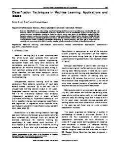
scales’ columns in Figure 5). Note that during the granularity level info propagation phase the next level feature set is extended after the feature selection phase therefore they are considered by the clustering methods for sure. The introduced method can correctly recognize 83% of the flows on the packet level, 8% on segment level and 3% on flow level. VI. C ONSTRAINED CLUSTERING Constraint clustering is a state-of-the-art [5],[6] technique to improve clustering. The key idea is to describe constraints, which tell which instances must or must not be in the same cluster. Then the feature-space is transformed to fulfill the constraints as much as possible (see Figure 7). It is important to note that constraint clustering can improve the feature selection deficiencies as well (it improves features in a similar way as in Principle Component Analysis [28]). A. Introduced constraints In our system, we introduced constraints providing information about the flow instances from independent traffic classification methods. Note that we only propose must constraints. It is important that constraints must not introduce error to the system. To achieve this we use only simple and strong heuristics. The introduced must constraints are always defined between flows with the same label. We propose to use the following three constraints (defined for flows being around the same time) •

•

Constraint Type 1 (red, row/col (1,3); (1,5); (2,3); (2,5)): Flows originating from different srcIPs going to the same dstIP (if we know they are both P2P, we can be sure they are the same app client (factor #1), as well, such as Azureus or uTorrent) Constraint Type 2 (orange, row/col (1,3); (1,4); (3,3); (3,4); (4,3); (4,4)): Flows originating from the same srcIP from the same srcPorts (and same for dst) (flows

75

ICN 2012 : The Eleventh International Conference on Networks

proto TCP TCP TCP TCP TCP TCP

srcIP srcPort dstIP dstPort label A B C D P2P E F C G P2P A B H I P2P A B J K P2P A L M N P2P A L M N P2P

95

avg througput [Mbps] Constraints

1 1 2 1 0.2 5

94.5

1 2 1 3 1 4 5 6

94 TP [%]

Flow ID 1 2 3 4 5 6

93.5 93 92.5 92 0

200

400

600

800

Constraints# Port

Fig. 8.

•

Connection pattern

DPI

Traffic characteristics

Fig. 9. TP ratio in the function of used constraints /Leftmost square: TP ratio without constraints, dot line: trendline/

Introduced constraints

from the same IP:port share both application and client program (factors #1 and #3), as well) Constraint Type 3 (yellow, row/col (5,3); (5,8); (6,3); (6,8)): Flows with significantly different traffic characteristics with the same user IP address (different characteristics imply different network conditions, factor #5)

one level to be fed to a lower granularity level. In this step a further 5% is gained relative to the previous step. Third, we introduced constraint clustering based on connectivity patterns. This resulted in a 2% increase of accuracy. The overall accuracy of the system on a mix of real world network traffic is 94% which is a 9-10% increase in accuracy comparing to state-of-the-art algorithms. ACKNOWLEDGMENT

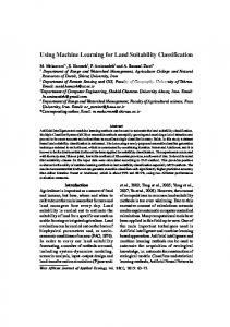
B. Evaluation Figure 9 shows the TP ratio in the function of used constraints. In general, a huge number of constraints could be collected, e.g., for each of the flows which take part in the definition of a type 2 constraint can be constructed a constraint. As increasing the number of constraints increases the run time of the constraint clustering algorithm a lot, the constraints are sampled in practice. The two extreme cases are easy to interpret: it is better to use constraints than not, and it is also very clear that increasing the number of constraints does not imply the increase of TP ratio directly. In the right corner of Figure 9 the TP ratio shows a big variance around the application of 600-1000 constraints. What can be learned from these experiments is that it is advisable to add more and more constraints iteratively during the model construction phase and evaluate whether it increased the overall accuracy or not. It is possible to achieve even 2% gain in TP ratio with a limited number of constraints. The detailed study of the variance of the accuracy in the function of the introduced constraints can be the focus of a further work. VII. C ONCLUSION In this paper, we introduced several steps to improve the current state-of-the-art in traffic classification engines relying entirely on packet header data. To become robust our proposed method incorporates clustering and classification methods. This way our method performs well even under changing network conditions. In this step we gained 3% TP ratio compared to standalone clustering or classification methods. In the second step, we proposed to perform the data collection on several granularity levels and the results of

Copyright (c) IARIA, 2012.

ISBN: 978-1-61208-183-0

J´anos Sz¨ule thanks the partial support of the EU FP7 OpenLab project (Grant No.287581), the National Development Agency (TAMOP 4.2.1/B-09/1/KMR-2010-0003) and the National Science Foundation OTKA 7779 and 80177. R EFERENCES [1] M. Pietrzyk, J.-L. Costeux, G. Urvoy-Keller, and T. EnNajjary, “Challenging Statistical Classification for Operational Usage: The ADSL Case,” in IMC ’09: Proceedings of the 9th ACM SIGCOMM conference on Internet Measurement Conference. New York, NY, USA: ACM, 2009, pp. 122–135. [2] A. W. Moore and D. Zuev, “Internet Traffic Classification Using Bayesian Analysis Techniques,” in Proc. SIGMETRICS, Banff, Alberta, Canada, June 2005. [3] A. McGregor, M. Hall, P. Lorier, and A. Brunskill, “Flow Clustering Using Machine Learning Techniques,” in Proc. PAM, Antibes Juan-les-Pins, France, April 2004. [4] F. Palmieri and U. Fiore, “A Nonlinear, Recurrence-based Approach to Traffic Classification,” Comput. Netw., vol. 53, pp. 761–773, April 2009. [5] M. Bilenko, S. Basu, and R. J. Mooney, “Integrating Constraints and Metric Learning in Semi-supervised Clustering,” in ICML ’04: Proceedings of the twenty-first international conference on Machine learning. New York, NY, USA: ACM, 2004, p. 11. [6] S. Basu, “Repository of Information on Semi-supervised Clustering,” retrieved: Oct, 2011. [Online]. Available: http://www.cs.utexas.edu/users/ml/risc/code/ [7] J. Erman, M. Arlitt, and A. Mahanti, “Traffic Classification Using Clustering Algorithms,” in Proc. MineNet ’06, New York, NY, USA, 2006.

76

ICN 2012 : The Eleventh International Conference on Networks

[8] N. Williams, S. Zander, and G. Armitage, “A Preliminary Performance Comparison of Five Machine Learning Algorithms for Practical IP Traffic Flow Classification,” SIGCOMM Comput. Commun. Rev., vol. 36, no. 5, pp. 5–16, 2006.

[22] D. H. Fisher, “Knowledge Acquisition via Incremental Conceptual Clustering,” Machine Learning, vol. 2, pp. 139–172, 1987, 10.1007/BF00114265. [Online]. Available: http://dx.doi.org/10.1007/BF00114265

[9] L. Jun, Z. Shunyi, X. Ye, and S. Yanfei, “Identifying Skype Traffic by Random Forest,” in WiCom ’07: Proceedings of the 3rd International Conference on Wireless Communications, Networking and Mobile Computing, Sept. 2007, pp. 2841 – 2844.

[23] M. S. L. Ertoz and V. Kumar, “A New Shared Nearest Neighbor Clustering Algorithm and Its Applications,” in Workshop on Clustering High Dimensional Data and its Applications at 2nd SIAM International Conference on Data Mining, 2002.

[10] R. Bar-Yanai, M. Langberg, D. Peleg, and L. Roditty, “Realtime Classification for Encrypted Traffic,” in Proc. SEA, 2010, pp. 373–385. [11] A. W. Moore, M. L. Crogan, and D. Zuev, “Discriminators for Use in Flow-based Classification,” Tech. Rep., 2005. [12] J. H. Plasberg and W. B. Kleijn, “Feature Selection Under a Complexity Constraint,” Trans. Multi., vol. 11, no. 3, pp. 565–571, 2009. [13] A. Este, F. Gringoli, and L. Salgarelli, “Support Vector Machines for TCP Traffic Classification,” Comput. Netw., vol. 53, pp. 2476–2490, September 2009. [Online]. Available: http://dl.acm.org/citation.cfm?id=1576850.1576885 [14] A. Yang, S. Jiang, and H. Deng, “A P2P Network Traffic Classification Method Using SVM,” in Young Computer Scientists, 2008. ICYCS 2008. The 9th International Conference for, nov. 2008, pp. 398 –403.

[24] R. H. John Stutz and P. Cheeseman, “Bayesian Classification Theory,” NASA Ames Research Center, 1991, Tech. Rep. [25] C. Cortes and V. Vapnik, “Support-Vector Networks,” Mach. Learn., vol. 20, pp. 273–297, September 1995. [26] T. Auld, A. W. Moore, and S. F. Gull, “Bayesian Neural Networks for Internet Traffic Classification,” IEEE Transaction on Neural Networks, vol. 18, pp. 223–239, 2007. [27] W. E. Leland, M. S. Taqqu, W. W., and D. V. Wilson, “On the Self-Similar Nature of Ethernet Traffic (Extended Version),” IEEE/ACM Transactions on Networking, vol. 2, pp. 1–15, 1994. [28] K. Pearson, “On Lines and Planes of Closest Fit to Systems of Points in Space,” The London, Edinburgh and Dublin Philosophical Magazine and Journal of Science, Sixth Series, vol. 2, pp. 559–572, 1901.

[15] L. Bernaille, R. Teixeira, I. Akodkenou, A. Soule, and K. Salamatian, “Traffic Classification On The Fly,” SIGCOMM Comput. Commun. Rev., vol. 36, no. 2, pp. 23–26, 2006. [16] E. Hjelmvik and W. John, “Statistical Protocol IDentification with SPID: Preliminary Results,” in SNCW 2009: 6th Swedish National Computer Networking Workshop, May 2009. [17] G. G. Sena and P. Belzarena, “Early Traffic Classification Using Support Vector Machines,” in Proceedings of the 5th International Latin American Networking Conference, ser. LANC ’09. New York, NY, USA: ACM, 2009, pp. 60–66. [Online]. Available: http://doi.acm.org/10.1145/ 1636682.1636693 [18] “Ericsson Network Performance Partnership Tools,” retrieved: Oct, 2011. [Online]. Available: http://www.ericsson.com/ourportfolio/telecom-operators/ network-performance-partnership?nav=marketcategory002 [19] “Weka 3: Data Mining Software in Java,” retrieved: Oct, 2011. [Online]. Available: http://www.cs.waikato.ac.nz/ml/weka/ [20] “Rapidminer,” retrieved: Oct, 2011. [Online]. Available: http://www.rapidminer.com/ [21] S. Zander, T. Nguyen, and G. Armitage, “Automated Traffic Classification and Application Identification Using Machine Learning,” in Proc. IEEE LCN, Sydney, Australia, November 2005.

Copyright (c) IARIA, 2012.

ISBN: 978-1-61208-183-0

77