The CSI Journal on Computer Science and Engineering (JCSE) - Submitted
1
Multi-Sensor Fuzzy Data Fusion Using Sensors with Different Characteristics Mohammad Amin Ahmad Akhoundi1, Ehsan Valavi2 • Abstract – This paper proposes a new approach to multisensor data fusion, suggesting by considering information about the sensors’ different characteristics, aggregation of data acquired by individual sensors can be done more efficient. Same as the most effective sensors’ characteristics, especially in control systems, our focus is on sensors’ accuracy and frequency response. A rulebased fuzzy system is presented for fusion of raw data obtained from the sensors having complement characteristics in accuracy and bandwidth. Furthermore, a fuzzy predictor system is also suggested aiming to extremely high accuracy for highly sensitive applications. The great advantages of the proposed sensor fusion system are revealed on simulation results of a control system utilizing the fusion system for output estimation. Index Terms – Sensor fusion, Fuzzy Control.
I. INTRODUCTION
M
EASUREMENT is a significant requirement for today’s industrial world. Applications such as control, safety and monitoring systems are inseparable parts of industry. It is not possible to imagine such applications without sensing systems. The more advances are made in industries, the more demands for more accurate measurement systems could be observed. Many parameters are in play here, however, the main contributor in which restricts the performance of these systems in many cases is lack of sensors that meet our requirements. In fact, sensors have some characteristics which limit range of their applications. Two important instances of mentioned characteristics are accuracy and frequency response of a sensor. These restrictions originate from the physical features of a sensor and can be observed due to some fabrication problems or where renewing or changing old sensors are not economically justifiable. However, hardware limitations in many cases can be almost compensated using software solutions. Sensor-fusion is a software approach for improving reliability of information obtained from a sensory system using aggregation of multiple sensors’ information. Aggregated information also refers to optimal or maximum information [1], conveys valuable and reliable data that cannot explicitly be found in primary sensor values. Actually, sensorfusion masks errors and erasures coming from individual sensors and leads to better and more accurate estimation of the measured variable. Fusion methods can be categorized into three major clusters listed here. 1 2
University of Tehran, (email:
[email protected] ) Institute for Research in Fundamental Sciences (IPM) (email:
[email protected])
• •
Probabilistic methods such as Bayesian analysis of sensor values, Evidence Theory, Robust Statistics, and Recursive Operators. Least square-based estimation methods such as Kalman Filtering, Optimal Theory, Regularization, and Uncertainty Ellipsoids. Intelligent aggregation methods such as Neural Networks, Genetics Algorithms, and Fuzzy Logic.
In most of the works done in this area, all of the sensors have been treated in a same way, i.e. no well-defined differences in sensor’s performance characteristic are considered. In this research we are going to propose a fuzzy intelligent method for sensor fusion which is mainly based on information about sensor’s characteristics. We specially concentrate on accuracy and bandwidth of an ordinary sensor as the parameters having the most effects on the performance of a sensory system. Many Applications require sensors with high accuracy and also enough sensitivity in response to rapid and high-frequency changes in the measured variable. In some cases such a sensor is not easily available or using it is not economically justifiable. Our solution is based on aggregation of information from sensors with complement characteristics in accuracy and bandwidth, in order to have an acceptable estimation of the measured variable that meets our requirements. In spite of many other methods, the presented fusion algorithm does not need the system’s model which the measured variable belongs to. It only depends on some general information about accuracy and bandwidth of the sensors. Because of the fact that the problem of inaccuracy and slowness of sensors appears mostly in industrial control systems, our focus is on control and monitoring applications. The rest of this paper is organized as follow. A summarized literature review is presented at Section II. The problem exactly is defined in Section III. In that section we also introduce our method and explain its two different in detail. Simulation of the method in a control system benchmark and discussion about its results is the contents of Section IV. Finally, Section V provides conclusion and other comments about the research. II. RELATED WORKS A complete survey of information fusion techniques for reliable data fusion can be found at [2], however, sensor fusion problems, applications, and future directions are completely addressed at [3,4,5,6,7]. As it can be grasping from contents of mentioned papers, industries requirement forced
The CSI Journal on Computer Science and Engineering (JCSE) - Submitted researchers to propose more precise, yet feasible, algorithms for sensor fusion. Consequently, we can see many application oriented use of sensor fusion in the literature. A case in point, in [8] they mainly concentrate on reducing redundancy and noise and also attempt to improve failure tolerability of information generated by sensors of gas turbine power plants. More practical and industrial application of sensor fusion can be found at [9, 10, 11, 12]. Those precise mathematical algorithms lead through the way of using probability models, evolutionary methods, and intelligent decision making means as discussed and categorized previously. An optimal linear fusion framework was proposed in [13] for addressing and solving measurement systems’ problems. In [14], authors consider two-sensor signal enhancement problem in a noisy environment. Their proposed solution is based on expectation maximization algorithm for jointly estimating the main signal, the coupling system and the unknown signal and noise parameters. [15] presents a systematic scheme for generating optimum fusion rules, which reduce computational tremendously compare to ordinary exhaustive search. In [16], two novel neural data fusion algorithms based on a linearly constrained least square (LCLS) method are proposed. Early attempts for recruiting fuzzy rules in multisensory data fusion can be seen at [17]. Inspired by their opinions, other researchers use fuzzy rules for overcoming mathematical approaches’ shortcomings in proposing practical solutions. For instance, a fuzzy-based multi-sensor data fusion classifier is developed and applied to land cover classification using ERS1/JERS-1 SAR composites in [18]. In addition to using fuzzy rules, some researches such as [19, 20] have tried to introduce new fuzzy logic operators in order to utilize intuitive knowledge about a system for sensor-fusion. In a practical problem, to correct slow sensor drift faults, [21] presents a hybrid method using fuzzy logic and genetic algorithm. In order to exploit advantages of both fuzzy-logic as an outstanding intelligent method, and Kalman filter as an efficient fusion method, [22] suggests a hybrid Kalman filterfuzzy logic adaptive multisensor data fusion architectures. In most of these researches, no clear differences between sensors are considered; however, sensors have certain known characteristics describing their behavior. Naturally, using information about these characteristics can lead to better designs for sensor fusion algorithms. The results may be more robust if, instead of using algorithms depending on system’s model, we only take advantages of methods considering sensor characteristics. III. PROPOSED METHODS A. Problem Statement The general goal of the system is to measure physical variable as accurate as possible. We use a wideband sensor that is not accurate enough to be used in a single manner (S1) and also a more accurate sensor with lower bandwidth (S2). The sensors utilized for a control system. The role of proposed method is to aggregate information obtained from these two types of sensors to best estimate the physical variable as a feedback for control purposes.
2
S1
Fuzzy Predictor: FP
S2
Fuzzy Aggregator: FA Output Z-1 Z-2
Z-n Fig. 1, The General Structure of SensorFusion Method
B. The General Structure of Sensor-Fusion Method The system uses a general structure described in figure 1. The Fuzzy Aggregator is the main part of the system. In a realtime process, it uses the sampled data from S1 and S2 to produce an estimation of the measured variable. It may also use another input from Fuzzy Predictor for better estimation. Fuzzy Predictor (FP) used n prior samples of estimated values for predicting the upcoming value. Although there are potentials for using FP because of its great benefits in applications needed an extreme accuracy, it is not essentially required to use in all applications owing to complexity in calculations leading to problems in real-time processing. Therefore, in many applications Fuzzy Aggregator can be used without Fuzzy Predictor. C. Fuzzy Aggregation First of all, not considering Fuzzy Aggregator’s predicted input, we can deal with only S1 and S2. A weighted average of S1 and S2 can provide an appropriate estimation of measured variable, if the weight of each sensor is determined appropriately. ,
1
Fuzzy aggregator (FA) determines weight of each sensor in (1) through a rule-based fuzzy system. Assuming the sensors’ weights are normalized, the fuzzy system is required to calculate only the weight of S1 as the output. Differential of S2 measurement and difference between S1 and S2 values are selected as the two inputs of the fuzzy system. Differential of S2 through boost of high frequency components, regains some of the signal’s information lost by the low-bandwidth sensor.
The CSI Journal on Computer Science and Engineering (JCSE) - Submitted
rate of measured variable is high, but the difference of values of S1 and S2 is still low. We need a new variable as another output of Fuzzy Aggregator to compensate this error. The output variable called “drift” is an estimation of the amount of error and is added or subtracted from the final estimation according to the slope of changes in the measured variable. The structure which is required for this operation can be described in figure 3. The fuzzy rule that we can obtain from these linguistic analysis can be expressed as below:
0.015 Ideal Sensor S2 S1
0.01 0.005 0 -0.005 -0.01 -0.015
Drift should be large only when: is small and If
-0.02 -0.025 -0.03
3
1
1.2
1.4
1.6
1.8
2
2.2
2.4
2.6
2.8
3
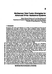
Fig. 2, Comparison between values of S1 and S2
It also provides an appropriate value for judging about the rate of changes in measured variable, because of its low noise. Due to its inaccuracy, S1 can give misleading information about the signal’s changes, but its difference with value measured by S2 can give some information about the reliability of S1 in situations with low changes in value of S2. For determining the weights if each sensor, we must use the system’s inputs appropriately. S1 must have a greater weight, when the changes in the measured variable are rapid, and these changes cannot appear in output of S2 due to its slow response. Also when the variable does not have rapid alternations and changes in a smooth way, the weight of S2 should be greater to prevent the uncertainty of S1 from affecting on the estimation. On the other hand, if the slope of changes in the measured variable is slow, and the difference between the values of S1 and S2 is large, it is because of high inaccuracy of S1, and therefore its weight should be highly reduced. In the case of high changes in the measured variable and also high difference between two sensors’ values, it can be concluded that the mentioned difference has happened because of the slow response of S1; therefore, weight of S1 should be very large. These inferences can be expressed as fuzzy rules below: is small and If Then: W1 should be small.
/
is small,
is small and If Then: W1 should be large.
/
is large,
is large and If Then: W1 should be very small.
/
is small,
If is large and Then: W1 should be very large.
/
is large,
/
is large.
Table.1 completely presents obtained fuzzy rules. As the “common sense” fuzzy rules are obtained, appropriate membership functions for linguistic variables used in the fuzzy rules should be defined. Figure 4 shows selected membership functions. The domain of functions definitions depend on the expected range of changes in the measured variable. Inputs Abs(S1-S2) Abs(dS2/dt) S S S G G S G G
W1 S G SS GG
Outputs Drift S G S S
Table 1, Fuzzy Rules
Fig. 3, General Structure of the Rule-Based Fuzzy System Abs (S1-S2)
Abs (dS2/dt)
In addition to w1, the fuzzy system should have also another output. The weighted average will be an appropriate estimation, only if the real signal lies between the two sensors’ values. There are situations in which error in value of S1 leads both values associated with S1 and S2 to be placed in one side of the real signal. Such a situation is more “probable” when
The CSI Journal on Computer Science and Engineering (JCSE) - Submitted W1, Weight of S1
defined according to the type of the application. If the result of the check exceeds the level, it should be ignored; otherwise the arithmetic average of its value and the output of rule-based fuzzy system should be considered as the final output of the Fuzzy Aggregator system. The figure 5 shows the exact and complete structure of the Fuzzy Aggregator system.
Drift
Fuzzy Prediction
Fig. 4, Membership functions for inputs and outputs of the system
Predicted Input
S1
S2
Rule-Based Fuzzy System
1) The System’s Overview From the conceptual perspective, designing fuzzy systems based on input-output data can be divided into two different categories of methods. In the first methods, the fuzzy system is designed based on the fuzzy rules obtained from the inputoutput data. Designing the Fuzzy Aggregator (FA) has been done from such a perspective. But the Fuzzy Predictor uses the second method. It suggests choosing an appropriate structure for the system (naturally including some parameters), and then optimizing the parameters using an appropriate training algorithm.
The Fuzzy Predictor system is an intelligent system with n inputs, which are n previous consecutive samples of the Fuzzy Aggregator’s outputs. The system’s structure can be expressed are “n” previous samples. in (2). In the formula , … ,
Fuzz y Aggr egato r
4
Checking Prediction Validity
Arithmetic Average
,…,
2
In each sampling period, which is a training step, the system’s parameters are modified aiming to achieve closer estimation of to . Using this online training , ,…, algorithm we have an extrapolation that is , ,…, , predicting the next sample of the measured variable. After passing enough training steps, the prediction can be reliable. 2) Gradient Descent Algorithm
Final Output Fig. 5, General Scheme of Fuzzy Aggregator A
Now what is the role of the predicted input? It is an input for improving the fuzzy fusion system’s performance. The way by that its value should be obtained, is explained in the next section. The key fact here is that it is not always reliable because it is just a prediction. In environments with strongly changing, repeated, and stochastic disturbances, the predictor is not very useful. However, in systems needing an extreme amount of accuracy (even at the expense of complexity of calculations) and also with smoothly changing disturbances, the fuzzy predictor can be beneficial. In the time ranges of happening disturbances, the predictor might be wrong. We can compare the prediction with the output of fuzzy system, as depicted in the figure 5, to check the validity of the prediction. The most level of tolerated difference between the predicted value and the output of the rule-base fuzzy system should be
There is a function and is a vector with some elements. The function includes some unknown parameters, , , . . . . It is required that at a certain point , becomes as small as possible, by choosing optimal values for unknown parameters of . The gradient descent algorithm suggests a method to achieve this goal. It expresses by choosing appropriate initial values for , , . . . , each parameter in each algorithm step should be modified according to (3) until the remains constant in two consecutive steps. 1
3
The symbol demonstrates the training step and is a constant representing length of each step. It should be small enough to lead to convergence of algorithm.
The CSI Journal on Computer Science and Engineering (JCSE) - Submitted 3) Fuzzy Predictor Using Gradient Descent By choosing different forms of the system’s membership functions, we can obtain different classes of the fuzzy systems. If we choose multiplying inference engine, singletone fuzzifier, center average deffuzifier, and Gaussian membership functions, the general form of such a system can be written in the close-form expression (4). ∏
∑
exp 4
∑
∏
exp
In which input x is a vector including n inputs of the system. The output f is also the prediction of the “upcoming sample” of the signal. Also the parameter M demonstrates the number of rules. Such a structure has the capability of showing intelligent behaviors due to fuzzy systems’ intrinsic features. The system’s unknown parameters are: 1,2 … 1,2 … , 1,2, … 1,2 … , 1,2, … Considering following definitions we can write the expression more simple.
exp
5
, /
6 7
In each sampling period, the goal of the system is minimizing the error defined in (8). 1 8 , ,…, 2 According to gradient descent method in each training step we should modify the parameter in this general way: 1
9
Using (4-7) we can obtain recurrence expressions required to modify systems’ parameters in each training step: 1
10
1
11
1
12
The modification of parameters according to (10-12) continues until the amount of error (e) becomes less than a threshold
5
value. Then the predicted value as the output of the system will be calculated as (13). , ,…, 13 In the next sampling period the same algorithm will be done by the new stet of inputs. IV. SIMULATION AND RESULTS Accuracy and speed of a measurement system highly affects the performance of control systems. If the feedback provided for a control system is not accurate and rapid enough, the system will fail to regulate the output properly. Choosing inappropriate sensors also may lead to the system’s oscillation and even its instability. Because of the significant role of measurement systems in control applications, our focus for assessing the fusion method is on evaluation of response of the control system which uses it. As a benchmark we have chosen an inverted pendulum control system for evaluation of the proposed measurement system. Figures 6 through 18 show response of the control system and also outputs of the fuzzy system designed for sensor fusion. The system has an initial condition and is required to set the output at zero. A disturbance, also, is applied to the system after 25 seconds. Using an ideal sensor causes the response of the system to be similar to what is shown as figure 6. But if we use just sensor S1 as the feedback, the response of the system is the same as what is shown in figure 7. The inaccuracy of the sensor causes high deviation of the response from the zero line. Use of a slow sensor as S2 can lead to an oscillatory response as depicted in the figure 8. If we use an ordinary average to combine both information in S1 and S2 a response such as figure 9 could be obtained. This illustrates those a simple method for aggregation in which weights of sensors are equal in all the time, is not efficient, and consequently, more intelligent method is required to have an acceptable response. In previous sections, it was mentioned that the fuzzy system including a rule-based fuzzy system (that is a part of fuzzy aggregator in presence of predicted input) and a fuzzy predictor can be used for having an accurate estimation of the measured variable. It was claimed that in many applications the fuzzy aggregator system can be the sole system used for fusion. The system has two outputs: W1 which is weight of S1 and also Drift. The former is the main output of the system, and the latter is used to compensate probable errors that may happen in such a system. We discussed that the system without the Drift output results in unacceptable performance. This fact can be observed in the figure 10, where the response of the system with the fuzzy aggregator without Drift output is shown. But the complete Fuzzy Aggregator system (with both Drift and W1 outputs) even without the fuzzy predictor system can help us achieve an appropriate response according to the figure 11. Figures 12 and 13, show the changes of the two outputs of Fuzzy Aggregator. Figure 14 compares the real signal and values of S1 and S2. It can be observed that the sensor S1 has not only considerable deviations, but also a negative average drift relative to the main signal. Figure 15 illustrates how the fusion method estimates real amount of the measured variable.
The CSI Journal on Computer Science and Engineering (JCSE) - Submitted
0.02
6
0.08 0.06 0.04
Output Angle (Rad)
Output Angle (Radian)
0
-0.02
-0.04
-0.06
0.02 0 -0.02 -0.04 -0.06 -0.08
-0.08
-0.1
-0.1
0
5
10
15
20
25
30
35
40
45
-0.12
50
0
5
10
15
20
Time (sec)
Fig. 6, The system’s output using ideal sensor 0.02
0.06
0
0.04
35
40
45
50
0.02
-0.02
Output Abgle (Rad)
Output Angle (Rad)
30
Fig. 10, The system’s output using fuzzy system’s output as the feedback without Fuzzy Predictor and also Drift output
0.04
-0.04 -0.06 -0.08 -0.1 -0.12
25
Time (sec)
0 -0.02 -0.04 -0.06 -0.08
0
5
10
15
20
25
30
35
40
45
50
Time (sec)
-0.1 -0.12
Fig. 7, The system’s output using sensor S1
0
5
10
15
20
25
30
35
40
45
50
Time (sec)
0.15
Fig. 11, The system’s output using fuzzy system’s output without predictor 0.1
0.8 0.7
0
0.6
-0.05
W1
Output Angle (Rad)
0.9 0.05
-0.1 -0.15 -0.2
0.4 0.3 0.2
0
5
10
15
20
25
30
35
40
45
50
0.1
Time (sec)
Fig. 8, The system’s output using sensor S2
0
0
5
10
15
20
25
30
35
40
45
Time (sec)
0.08
Fig. 12, W1, the weight of S1, output of fuzzy system
0.06
Output Angle (Radian)
0.5
0.04 0.02 0 -0.02 -0.04 -0.06 -0.08 -0.1 -0.12
0
5
10
15
20
25
30
35
40
45
Time (sec)
Fig. 9, The system’s output using ordinary average of S1 and S2 as the feedback
50
In order to have a more accurate estimation and naturally a better performance of control system we can use also Fuzzy Predictor system. In our simulation, we use 20 previous samples of estimated measured variable to predict the next one. The response of the system is shown on figure 16. Also the predicted output in each time is described in figure 17. The problem about Fuzzy Predictor is temporarily inaccurate prediction during happening of disturbances. The problem can be detected by the comparison of the prediction result and output of Fuzzy Aggregator system. In this situations the predicting system should temporarily ignored.
50
The CSI Journal on Computer Science and Engineering (JCSE) - Submitted -3
5
In this case, there are three parameters which can almost describe the behavior of sensors: Variance of deviations of the sensor S1, the average of its error, and the bandwidth or timeconstant of the sensor S2. We use two criteria defined in (14, 15) to evaluate the system performance under changes of these parameters.
x 10
4 3 2
Drift (Radian)
7
1 0
|
|
14
-1 -2
|
|
15
-3 -4 -5
0
5
10
15
20
25
30
35
40
45
50
Time(sec)
IAE is based on absolute error of system’s output over a certain period of time. ITAE is more sensitive to errors in steady state situation.
Fig. 13, “Drift” the output of rule-based fuzzy system
0.04 0.02
0.02 Output Angle (Rad)
0
Output Angle (Rad)
0 -0.02
Real Signal S2 S1
-0.04
-0.02 -0.04 -0.06
-0.06
-0.08
-0.08
-0.1
-0.1
-0.12
-0.12 -0.14
0
5
10
15
20
25 Time(sec)
30
35
40
45
50
Fig. 16, The system’s output using complete sensor-fusion algorithm with both fuzzy aggregator and fuzzy predictor 0
1
2
3
4
5
6
7
8
9
10
Time (sec)
0.04
Fig. 14, Comparison between main signal and two sensors’ values Predicted Output (Radian)
0.02
0.02 0 Real Signal Estimated Signal
Output Angle (Rad)
-0.02 -0.04 -0.06
0
-0.02
-0.04
-0.06
-0.08
-0.08
0
5
10
15
20
25
30
35
40
45
50
Time (sec)
-0.1
Fig. 17, Fuzzy Predictor’s Output -0.12
0
1
2
3
4
5 Time (sec)
6
7
8
9
10
Fig. 15, Comparison between f the main signal and its estimation
For evaluating the system’s performance efficiently, the response of the control system must be assessed in situations with sensors with different parameters and characteristics. In fact the sensor fusion system should be robust enough to give acceptable performance when the parameters of sensors slightly change. The characteristics of sensors are not certain and exact at all. We can model these characteristics approximately by a filter with a certain bandwidth or a source of noise with certain variance and arithmetic mean to show the uncertainty of sensors values. However, these models are not exact and constant. The characteristics of a sensor can have some changes over time. Therefore, the system must not highly depend on the sensors’ models.
Figure 18 shows IAEs resulted by the control system using sensors with different bandwidths for S2 and the sane sensor as S1. The fusion algorithm and its parameters have not altered with changes in bandwidth S2. The results have calculated corresponding to three different sensor processing’s methods: using only the S2 sensor, calculating arithmetic average of S1 and S2 as feedback, and using proposed sensor-fusion method. It can be observed that in all of the cases the fusion method leads to much less error. Whatever time constant the sensor S1 has had, using the single sensor or simple averaging has resulted in oscillation of the system. The similar results can be achieved by the figure 19 conveying ITAE values. The advantages of the method can get more revealed, when the criterion attaches more importance on steady state mode of the signal. Changing the second sensor’s variance of deviations,
The CSI Journal on Computer Science and Engineering (JCSE) - Submitted
8
the IAE and ITAE values will be the same as the figure 20 and 21 illustrates. We can observe completely acceptable performance of the sensor-fusion algorithm even with almost wide range of error associated with S1. The method could offer high advantages even when value of S1 includes an unknown constant drift according to figures 22 and 23. In fact, these results demonstrate robustness of the fusion method and its relative independence on sensor’s characteristics.
Fig. 21, ITAEs obtained by sensors with different deviation’s variance for S1
Fig. 18, IAEs obtained by sensors with different time constants for S2
Fig. 22, IAEs obtained by sensors with different error bias for S1
Fig. 19, ITAEs obtained by sensors with different time constants for S2
Fig. 23, ITAEs obtained by sensors with different error bias for S1
Fig. 20, IAEs obtained by sensors with different deviation’s variance for S1
The CSI Journal on Computer Science and Engineering (JCSE) - Submitted V. CONCLUSION We have presented a new approach to fuzzy sensor fusion. The approach considers different characteristics of utilized sensors. Concentrating on accuracy and bandwidth, as the two most important and influential parameters of a sensor, we have suggested a fuzzy method for two-sensor data fusion. It contains two different parts: Fuzzy Aggregator and Fuzzy Predictor in which Fuzzy Aggregator takes advantages of a fuzzy system with appropriate fuzzy inputs, membership functions, and fuzzy rules. We have discussed that the system can lead to an acceptable result in many applications, but if the application requires extreme degree of certainty and accuracy, Fuzzy Predictor can be very useful. However, it involves more complex calculations. Because of the great effects of measurement systems in control applications, we have evaluated the performance of our method through analyzing results of a control system – as a benchmark – utilizing the fusion method. However, the applications of the system are not restricted to control systems. By assessing response of the control system, we have discussed great merits of the fusion method and its robust performance.
[8]
REFERENCES
[16]
[1]
[2]
[3] [4] [5]
[6]
[7]
C. Son, “Optimal Control Planning Strategies with Fuzzy Entropy and Sensor Fusion for Robotic Part Assembly Tasks”. International Journal of Machine Tool & Manufacture, Vol. 42, 2002, pp. 1335-1334. H. Lee, K. Park, and R. Elmasri, “Fusion Techniques for Reliable Information: A Survey”, International Journal of Digital Content Technology and its Application, accepted, to appear. P. Varshney, “Multi-sensor data fusion,” Electronics and Communication Engineering Journal, Vol. 9, No. 6, 1997, pp. 245-253. D. L. Hall and J. Llinas, “An introduction to multisensor data fusion,” the IEEE, Vol. 85, No. 1, 1997, pp. 6-23. R. Luo, C. Yih, and K. Su, “Multisensor fusion and integration: approaches, applications, and future research directions,” IEEE Sensors Journal, Vol. 2, No. 2, 2002, pp. 107-119. D. Mandic, D. Obradovic, A. Kuh, T. Adali, U. Trutschel, M. Golz, P. Wilde, J. Barria, A. Constantinides, and J. Chambers, “Data fusion for modern engineering applications: An overview,” Intl. Conf. on Artificial Neural Networks (LNCS), Vol. 3697, 2005, pp. 715-721. D. Macii, A. Boni, M. D. Cecco, and D. Petri, “Tutorial 14: Multisensor
[9]
[10]
[11]
[12]
[13]
[14]
[15]
[17]
[18]
[19]
[20] [21]
[22]
9
data fusion,” IEEE Instrumentation and Measurement Magazine, Vol. 11, No. 3, 2008, pp. 24-33. K. Goebel, A. Agogino, “Fuzzy Sensor Fusion for Gas Turbine Power Plants,” Proceedings of SPIE, Sensor Fusion: Architectures, Algorithms, and Applications III, 1999, pp. 52-61. H. Hu, S. Qian, J. Wang, and Z. Shi, “Application of information fusion technology in the remote state online monitoring and fault diagnosing system for power transformer,” 8th Intl. Conf. on Electronic Measurement and Instruments, 2007, pp. 550-555. B. V Dasarathy. “Industrial Application of Multi-Sensor Information Fusion”. Proceedings of IEEE International Conference on Industrial Technology. January 2000. Y. Dongyong, Y. Yuzo, “Multi-sensor Data Fusion and its application to Industrial Control”, SICE 2000. Proceedings of the 39th SICE Annual Conference, 2000, pp. 215 – 220. D. Smith and S. Singh, “Approaches to multisensor data fusion in target tracking:A survey,” IEEE Trans. Knowledge Data Eng., vol. 18, no. 12, pp. 1696–1710, Dec. 2006. J. Zhou, Y. Zhu, Z. You, and E. Song, “An efficient algorithm for optimal linear estimation fusion in distributed multisensor systems,” IEEE Transaction on Systems, and Man and Cybernetics, Vol. 36, No. 2, 2006, pp. 1000-1009. E. Weinstein, A.V. Oppenheim, M. Feder, and J.R. Buck, “Iterative and sequential algorithms for multisensor signal enhancement,” IEEE Trans. on Signal Processing, vol. 42, no. 4, pp. 846–859, 1994. Y. Zhu and X. Rong, “Unified Fusion Rules for Multisensor multihypothesis network decision systems,” in Proc. 2003 IEEE Trans. Systems, Man, and Cybernetics, vol. 33, no 4, pp. 502-513, July 2003. H. Odeberg. “Fusing sensor information using fuzzy measures.”, Robotica, 1994, pp. 465-472. B. Solaiman, L. Pierce, and F. T. Ulaby, “Multisensor data fusion using fuzzy concepts: Application to land-cover classification using ERS1/JERS-1 SAR composites,” IEEE Trans. Geosci. Remote Sensing, vol. 37, May 1999, pp. 1316–1326. Y. S. Xia, H. Leung, and E. Bossé, “Neural data fusion algorithms based on a linearly constrained least square method,” IEEE Trans. Neural Netw., vol. 13, no. 2, Mar. 2002, pp. 320–329. J. Stover, D. Hall, and R. Gibson. “A fuzzy-logic architecture for autonomous multisensor data fusion”. IEEE Transactions on Industrial Electronics, vol.43, no3, 1996, pp.403–410. B. Karlsson, “Fuzzy measures for sensor data fusion in industrial recycling.” Meas. Sci. Technol., vol.9, 1998, pp.907-912. K. Goebel, W. Yan, "Hybrid Data Fusion for Correction of Sensor Drift Faults," Computational Engineering in Systems Applications, IMACS Multiconference on , vol.1, Oct. 2006, pp.456-462. P. J. Escamilla-Ambrosioand N. Mort, “Hybrid Kalman Filter-Fuzzy Logic Adaptive Multisensor Data Fusion Architecture”,. Proc. of The IEEE Conference on Decision and Control, 2003, pp. 5215-5220.