MAGNITUDE ESTIMATION USING GENERALIZED GAMMA PRIOR DISTRIBUTION. Tran Huy Datâ. Institute for Infocomm Research, Singapore.
MULTICHANNEL SPEECH ENHANCEMENT BASED ON SPEECH SPECTRAL MAGNITUDE ESTIMATION USING GENERALIZED GAMMA PRIOR DISTRIBUTION Tran Huy Dat∗
Kazuya Takeda, Fumitada Itakura
Institute for Infocomm Research, Singapore
Nagoya University, Japan
ABSTRACT We present multichannel speech enhancement method based on MAP speech spectral magnitude estimation using a generalized gamma model of speech prior distribution, where the model parameters are adapted from actual noisy speech in a frame-by-frame manner. The utilization of a more general prior distribution with its online estimation is shown to be effective for speech spectral estimation. We tested the proposed algorithm in an in-car speech database and obtained significant improvements on the speech recognition performance, particularly under nonstationary noise conditions such as music, air-conditioner and open window.
and speech enhancement system. The paper is organized as follows. In the next section, we introduce the multichannel model and assumptions used in this study. In Sec.3, we derive the multichannel MAP speech spectral magnitude estimation using the proposed model. In Sec.4, we describe algorithms to estimate the model parameters in a frame-by-frame manner. In Sec.5, we report the experimental evaluation. 2. MULTICHANNEL MODEL AND ASSUMPTIONS Consider the additive model of multichannel signals in the STDFT domain Xl (n, k) = Hl (n, k) S (n, k) + Nl (n, k) ,
1. INTRODUCTION Multichannel speech enhancement systems are widely used for hands-free communication and speech recognition. The most fundamental method is beamforming, where the positions of the target and noise sources are assumed to be apart or known in advance. Recently, statistical speech enhancement methods, extended from single-channel approaches, have been investigated [1]-[2] and have shown better results than beamforming. These methods model and estimate the distributions of speech and noise spectra, assuming the Gaussian model and then statistical estimators (MMSE or MAP) are employed. However, the Gaussian model, yielding an independence between magnitude and phase, is unnatural for speech signal [3]. Moreover, the noise field was assumed to be incoherent [1] which is also untypical in real conditions. Previously, we presented a generalized gamma model of speech prior distribution [3], where the distribution parameters are adapted from actual noisy speech. We have shown that, this method provides more accurate modeling of speech prior distribution and it improved the performance of single channel speech enhancement in terms of both sound quality and speech recognition. In this study, we extend this method for a multichannel approach. Furthermore, we develop a method to adapt the model parameters in a frame-by-frame manner. The motivation for this extension is that the multichannel systems, which can better distinguish the target signal from interfering noises, should improve the performances of the parameter estimation ∗ The
author was with Nagoya University, Japan.
142440469X/06/$20.00 ©2006 IEEE
T
(1)
T
where X = [X1 , ..., XD ] , N = [N1 , ..., ND ] are the vectors of the complex spectra of noisy and noise signals, H = T [H1 , ..., HD ] is the vector of transfer functions, S is clean speech spectrum and l = 1 : D is the microphone index. Couple (n, k) denotes the time-frequency index and will be omitted in Secs.2 and 3. The differences between our model and those proposed in [1]-[2] are as follows. -Due to a possible change in the positions of speakers, we do not assume transfer functions to be constant in each frequency bin. -The noise is assumed to be spatially coherent and the noise spectral components follow the zero-mean independent identical multi-variable Gaussian distribution with a full covariance matrix � � 1 T −1 , p (NR ) = 2πD/2 det(2C 1/2 exp −NR Cn NR n) � � (2) 1 T −1 p (NI ) = 2πD/2 det(2C )1/2 exp −NI Cn NI . n
p (NR , NI ) = p (NR ) p (NI ) ,
(3)
where (.)R , and (.)I denote the real and imaginary parts of the complex spectrum, respectively and C n is half of the covariance matrix (real and symmetrical). -Speech spectral magnitude |S| follows a generalized gamma distribution given as � � � � � �La−1 L |S| ba |S| p (|S|) = exp −b , (4) Γ (a) σS σS σS
IV 1149
ICASSP 2006
where σS2 denotes the variance of speech spectrum. (a, b, L) are distribution parameters but the system has� two�remain2 ing free parameters due to the normalization |S| = σS2 , where �.� denotes the expectation. This distribution is a superset of conventional models, including Gaussian, generalized Gaussian and gamma distributions and was used in our previous study for single-channel approaches [3]. 3. MULTICHANNEL MAP SPEECH SPECTRAL MAGNITUDE ESTIMATION USING GENERALIZED GAMMA MODEL For the proposed generalized gamma model, the MAP speech spectral magnitude estimation is preferable to use due to its simplicity in implementation and the effectiveness [3]. Unlike Lotter et al [1], we derive the estimation for the case of a spatially coherent noise using generalized gamma model of speech prior distribution. The multichannel MAP estimation equation Sˆ = arg max [p (|S| |X )] can be expressed as |S|
∂ {log [p (X| |S|)] + log [p (|S|)]} = 0. ∂ |S|
(5)
where ϕS denotes the phase of the clean speech spectrum and ¯ T C−1 ϕX - the phase of H n X. Integrating (10) over ϕ S , we obtain the conditional distribution of noisy speech magnitude as a multichannel version of the Rician distribution [3]. � � � T −1 � ∆ ¯ C X . ¯ T C−1 H |S|2 I0 2 |S| H p (X| |S|) = exp −H n
(11) Here, I0 is the Bessel function of the first kind, which can be approximated by 1 ex , x > 0. 2πx The first term in (5) is then derived as I0 (x) ≈ √
2 |S| 1 ∂ {log [p (X| |S|)]} = − 2 − + ∂ |S| Un 2S where Un2 =
(12)
¯ T C−1 X| |H n ¯ T C−1 H n H Un2
1 . ¯ T C−1 H n H
(6)
Note that here, we consider the transfer functions as deterministic variables, which will be estimated from observations. Two terms in right side of (6) can be denoted using (2) and (3) � � 1 T −1 , p (XR |SR , SI ) = 2πD/2 det(C 1/2 exp −YR Cn YR n) � � 1 T −1 p (XI |SR , SI ) = 2πD/2 det(C )1/2 exp −YI Cn YI , n (7) where YR = XR − HR SR + HI SI , (8) YI = XI − HR SI − HI SR . Substituting (7) and (8) into (6) yields the conditional distribution of the complex spectrum of noisy speech expressed as ⎧ ⎡ T −1 � 2 � ⎤⎫ ¯ Cn H S + S 2 − ⎬ H ⎨ R �I � T −1 ¯ Cn X S R − ⎦ , p (X|S) = Q (X) exp − ⎣ −2Re �H � ⎩ ⎭ ¯ T C−1 −2Im H n X SI (9) where Q (X) is independent of S and this term will be reduced with further estimation. Since C n is real and symmet¯ T C−1 rical the term H n H is real. The conditional distribution (9) can be transformed into magnitude and phase, using Jacobian transform, yielding � � � � 2 ¯ T C−1 − H H |S| − ∆ n T −1 2 p (X|ϕS , |S|) = exp ¯ Cn X cos (ϕX − ϕS ) −2 |S| H (10)
(14)
From (4), the second term in (5) is given by (La − 1) |S| ∂ {log [p (|S|)]} = − Lb L−1 . ∂ |S| |S| σS
From (3), p (X| |S|) can be factorized as
, (13)
3.2. Gain function
3.1. Derivation of multichannel Rician distribution
p (X|S) = p (XR |SR , SI ) p (XI |SR , SI ) .
n
(15)
Substituting (13) and (15) into (5) yields the estimation equation, which generally can be solved by the Newton-Raphson method. However, in this study, we consider the solution for the case of L = 2, which yields a closed-form solution and therefore is suitable in the implementation. The estimation equation is then derived as −G2 + �
G 1+
b ξ
�+
4a − 3 = 0. G
(16)
Here the gain function is ¯ T C−1 H H G = T n−1 |S| H ¯ Cn X
(17)
and the generalized priori and posteriori SNR are ξ=
T −1 2 σS2 ¯ Cn X . , γ = H 2 Un
(18)
4. ONLINE PARAMETER ESTIMATION 4.1. Noise covariance and transfer functions The noise covariance is initially estimated in each frequency bin using the first 250ms of observations. Then it is recursively updated, using voice activity detection (VAD), Cn (n, k) = � � T � ¯ (n, k) X (n, k) D1 αCn (n − 1, k) + (1 − α) Re X Cn (n − 1, k) D0 (19)
IV 1150
X
where D1 and D0 are hypotheses of speech presence and absence, α is a smoothing coefficient. Differently from those methods proposed in [1]-[2], we estimate the transfer function via priori SNR (i.e., short-term statistics). Not losing the generality, we assume H1 = 1.
VAD
(20)
D1
(22)
where Cx is the noisy speech covariance matrix, which is estimated as in (21) without the VAD. ¯ T (n, k) X (n, k) Cx (n, k) = αCx (n − 1, k) + (1 − α) X (23) Taking into account (20), the phase of the transfer function can be estimated using the first column of C x . 4.2. Online estimation of prior distribution parameter The main point of the proposed model is that the modeled distribution parameters are determined from actual noisy speech. Unlike the single channel system [3], here we use cross-channel statistics to perform the estimation in a frame-by-frame manner. Denote the noisy speech power as 2
2
2
Transfer function
Prior parameter
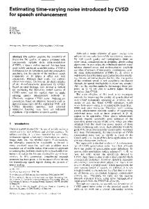
Fig. 1. Block-diagram processing
D0 (21) where χ is a smoothing coefficient. The priori SNR in the |H |2 σ2 i-channel ξi = σi 2 S is estimated by the decision-directed ni method [4]. The phase of the transfer function is estimated using the covariance matrix relationship ¯ T HσS2 + (Cn + jCn ) , Cx = H
Noise covariance Priori SNR Crosschannel statistic
The magnitude of the transfer function at microphone i is determined and smoothed as (n, k)| = |Hi� ⎧ � 2 (n,k) σn ⎨ 1 χ |Hi (n − 1, k)| + (1 − χ) ξξ1i (n,k) 2 (n,k) (n,k) σn i ⎩ |Hi (n − 1, k)| ,
Sˆ
Gain function
2
|Xi | = |Hi | |S| +|Ni | +2 |Hi | |S| |Ni | cos (∆φi ) , (24) where ∆φi is the phase difference, which is assumed to follow a uniform distribution [3]. Taking into account the independence of the phase and the magnitude of the noise spectrum, the cross-channel correlations of noisy speech power are expressed as � � � � � � 2 2 2 4 2 2 |X1 | |Xi | = |Hi | |S| + |N1 | |Ni | + � � �� � � � � 2 2 2 2 + |S| |Hi | |N1 | + |Ni | + 4 |Hi | |�N1 Ni �| , (25) �� � �� ��2 � 2 2 2 2 |Xi | = |Hi | |S| |X1 | + �� � � �� � � � �� � 2 2 2 2 2 2 |Ni | + |S| |Hi | |N1 | + |Ni | . + |N1 | (26)
Since all components in the lower term of (25) and (26) are given from transfer function, noise covariance matrix and priori SNR estimations, the ratio of the fourth to the secondmoments of |S| can be determined (at each time-frequency index). This ratio is used to ”match” the generalized gamma distribution parameters. For L = 2, yields [3] � � a (a + 1) �� 2 ��2 1 �� 2 ��2 |S| |S| |S| = = 1+ . b2 a (27) � � 2 = σS2 implies the relaNote that the normalization |S| � � � � 2 2 2 2 tionship a = b. The terms |X1 | |Xi | and |N1 | |Ni | are estimated using recursive moving averages as in (19) and (23). Finally, we smooth the estimated parameter as �
4
�
a (n, k) = µa (n − 1, k) + (1 − µ) a (n, k) ,
(28)
where µ is a smoothing coefficient. 4.3. Voice activity detection For VAD, we assume that the less noisy channel is known in advance. In addition to the conventional energy feature given from this channel, we use the cross-channel correlation coefficient ρ calculated from each frame to determine VAD. D
1 � ρ (n) = D − 1 i=2
|�X1 (n) Xi (n)�| �|X12 (n)|� �|Xi2 (n)|�
(29)
Here we assume that the channels have a higher correlation in the target signal durations. The resulting VAD is expressed as �
if |∆ (n)| > γ1 & ρ (n) > γ2 otherwise (30) where γ1 and γ2 are constant boosting factors. Currently γ 1 = 3 and γ2 = 0.3 are used. The energy distance ∆ is the ratio of current frame energy E 1 (n) to the stored-in-memory noise energy and is calculated in decibels. Unlike VAD, the noise energy is updated when |∆ (n)| > γ 1 . V AD (n) =
IV 1151
1 0
90
1 Input1
88
0
86 0
0.2
0.4
0.6
0.8
1
1.2
1.4
accuracy, [%]
−1 1
Input2 0 −1
0
0.2
0.4
0.6
0.8
1
1.2
1.4
1
82 80 78 76 74
Estimated parameter a in bin f=1kHz 0.5 0
84
72 70 0
0.2
0.4
0.6
0.8
1
1.2
Nearest mic.
1.4
1 Output
Single-channel LSA
Two-channel Single-channel psychoacoustic generalized gamma
Two-channel generalized gamma
0 −1
0
0.2
0.4
0.6
0.8
1
1.2
Fig. 3. Speech recognition overall performances on CIAIR in-car database
1.4
[s]
Fig. 2. Input 2-channel noisy signals (top two plots), example of estimated prior distribution parameter in bin f=1kHz (third plot) and output waveform (bottom) 5. EXPERIMENT We evaluate the proposed algorithm in CIAIR in-car speech corpus [5]. In the implementation, 16-kHz sampling signals from two microphones, attached to the ceiling [5] were used. The Hamming window of length of 20ms with 50% overlap was applied in FFT. Figure 1 shows the block diagram of processing. Given the multichannel noisy signals, VAD is performed using (30). Then noise covariance, priori SNR and cross-channel statistics are estimated using recursive averages. The transfer function is estimated using (21) and (22). The prior parameters are estimated and updated using (25)-(28). Then the gain function is given by (16)-(18). Finally, the phase adding and overlap and add are used to resynthesize the enhanced sounds. Examples of waveforms is plotted in Figure 2. Note that, the smoothing coefficients are chosen by hearing the output sounds. Currently, α = β = χ = 0.9, and µ = 0.6 are used. For reference, the EphraimMalah method (LSA), the single-channel version using generalized gamma modeling (GG) [3], and the multi-channel method based on psychoacoustic motivation (PA) [2] are also implemented. The overall results of speech recognition are shown in Figure 3. The proposed multichannel method is superior to others with approximately 16% improvement compared to the performance in the nearest microphone. The proposed method is particularly effective under nonstationary noise conditions. Table 1 shows the results for the cases of driving along an express way with a CD playing, high airconditioner (AC) and open window. The superiority of proposed methods can be explained by as follows. Firstly, using the more general distribution with its online estimation improves the accuracy of prior distribution modeling which is realized in the MAP estimation. Secondly, multi-channel systems improve the performance of VAD and parameter estimation. The online parameter estimation can also be considered as an optimization of the gain function, which controls the trade-off between noise reduction and distortion, resulting in the best speech recognition performance and the quality of enhanced sound which is confirmed by the listening test.
Table 1. Speech recognition rate on expressway under several driving conditions [%] Method Nearest 1-ch 1-ch 2-ch 2-ch mic LSA GG PA GG CD playing 82.27 82.61 85.62 83.96 92.98 High AC 51.00 87.33 89.00 88.67 91.67 Window open 42.67 76.67 78.33 77.33 86.33 6. CONCLUSIONS This study shows the effectiveness of using a more general prior distribution with online adaptation for multichannel speech enhancement. The accuracy of prior distribution modeling using multichannel observations is key point, which is realized in MAP speech spectral magnitude estimation. The experimental results show the superiority of the proposed method under nonstationary noise conditions. 7. REFERENCES [1] T. Lotter, C. Benien, and P. Vary, “Multichannel Direction-Independent Speech Enhancement Using Spectral Amplitude Estimation,” EURASIP Journal on Applied Signal Processing, vol.11, pp.1147-1156, 2003. [2] J. Rosca, R. Balan, and C. Beaugeant, “Multi-channel psychoacoustically motivated speech enhancement,” Proc. ICASSP, Hong Kong, 2003. [3] T.H. Dat, K. Takeda, and F. Itakura, “Generalized gamma modeling of speech and its online estimation for speech enhancement,” Proc. ICASSP, Philadelphia, USA, 2005. [4] Y. Ephraim and D. Malah, “Speech Enhancement Using a Minimum Mean-Square Error Short-Time Spectral Amplitude Estimator, ” IEEE Trans. ASSP, vol.ASSP32, pp.1109-1121, 1984. [5] K. Takeda, H. Fujimura, K. Itou, N. Kawaguchi, and S. Matsubara, “Construction and Evaluation of a Large In-Car Speech Corpus,” IEICE Trans.,vol.E88-D , pp. 553-561, 2005.
IV 1152