Multilevel Subspace Correction for Large-Scale Optimization Problems

UNIVERSITY OF CALIFORNIA Los Angeles

Multilevel Subspace Correction for Large-Scale Optimization Problems

A dissertation submitted in partial satisfaction of the requirements for the degree Doctor of Philosophy in Mathematics by Ilya A. Sharapov

1997

c Copyright by Ilya A. Sharapov 1997

The dissertation of Ilya A. Sharapov is approved.

Bjorn Engquist

Stanley Osher

Olivier Ledoit

Tony F. Chan, Committee Chair

University of California, Los Angeles 1997

ii

TABLE OF CONTENTS 1 Introduction : : : : : : : : : : : : : : : : : : : : : : : : : : : : : : : :

1

1.1 Background and Motivation : : : : : : : : : : : : : : : : : : : : : :

1

1.2 Recent Literature : : : : : : : : : : : : : : : : : : : : : : : : : : : :

5

1.2.1 Domain Decomposition Methods : : : : : : : : : : : : : : :

5

1.2.2 Subspace Correction for Optimization Problems and Nonlinear Problems : : : : : : : : : : : : : : : : : : : : : : : : : :

7

2 Subspace Correction Framework for Optimization Problems : : 10 2.1 Multiplicative Schwarz Method : : : : : : : : : : : : : : : : : : : :

10

2.1.1 Basic Method : : : : : : : : : : : : : : : : : : : : : : : : : :

10

2.1.2 Convex Problems : : : : : : : : : : : : : : : : : : : : : : : :

12

2.1.3 Nonconvex Problems : : : : : : : : : : : : : : : : : : : : : :

15

2.2 Coarse Grid Correction for Schwarz Methods : : : : : : : : : : : :

18

2.2.1 Asymptotic Convergence Rate : : : : : : : : : : : : : : : :

20

2.2.2 Convergence Rate for Additive Schwarz Methods : : : : : :

24

2.3 Constrained Optimization : : : : : : : : : : : : : : : : : : : : : : :

28

2.4 Multilevel Method : : : : : : : : : : : : : : : : : : : : : : : : : : :

34

3 Applications to PDE-Based Optimization Problems : : : : : : : 36 iii

3.1 Domain Decomposition Methods for Elliptic Eigenvalue Problems :

36

3.1.1 Subspace Correction for Eigenvalue Problems : : : : : : : :

37

3.1.2 Coarse Grid Correction and Multilevel Method : : : : : : :

48

3.1.3 Alternative Variational Characterization of the Smallest Eigenvalue : : : : : : : : : : : : : : : : : : : : : : : : : : : : : : :

51

3.2 Simultaneous Computation of Several Eigenvalues : : : : : : : : :

57

3.2.1 Generalization of the Rayleigh Quotient Minimization : : :

58

3.2.2 Subspace Correction for Simultaneous Computation of Several Eigenvalues : : : : : : : : : : : : : : : : : : : : : : : :

60

3.2.3 Numerical Examples on Unstructured Grids : : : : : : : : :

62

3.3 Graph Partitioning Using Spectral Bisection : : : : : : : : : : : : :

63

4 Applications to Optimization Problems Arising in Mathematical Finance : : : : : : : : : : : : : : : : : : : : : : : : : : : : : : : : : : : : : 71 4.1 Frobenius Norm Minimization for Multivariate GARCH Estimation 72 4.1.1 Problem Formulation and Numerical Solution : : : : : : : :

73

4.1.2 Numerical Examples : : : : : : : : : : : : : : : : : : : : : :

78

4.2 Factor Analysis Problem : : : : : : : : : : : : : : : : : : : : : : : :

79

4.2.1 Numerical Solution : : : : : : : : : : : : : : : : : : : : : : :

81

4.3 Gain-Loss Optimization : : : : : : : : : : : : : : : : : : : : : : : :

85

4.3.1 Problem Formulation : : : : : : : : : : : : : : : : : : : : : :

87

4.3.2 Dual Problem and Interior Point Algorithm : : : : : : : : :

90

iv

4.3.3 Subspace Correction and Gauss-Seidel Method : : : : : : :

95

Bibliography : : : : : : : : : : : : : : : : : : : : : : : : : : : : : : : : : : 101

v

LIST OF FIGURES 2.1 Theorem 2.3. : : : : : : : : : : : : : : : : : : : : : : : : : : : : : :

22

2.2 Theorem 2.5. : : : : : : : : : : : : : : : : : : : : : : : : : : : : : :

32

2.3 Possible convergence to a non-solution. : : : : : : : : : : : : : : : :

33

3.1 Algorithm 3.1 for 2D Laplacian without the coarse grid correction.

49

3.2 Algorithm 3.1 for 2D Laplacian with the coarse grid correction. : :

50

3.3 Airfoil grids for simultaneous computation of several eigenmodes. :

64

3.4 Simultaneous computation of four eigenmodes. 1067 nodes 35 subdomains. : : : : : : : : : : : : : : : : : : : : : : : : : : : : : : : : :

65

3.5 Simultaneous computation of four eigenmodes. 1067 nodes, 78 subdomains. : : : : : : : : : : : : : : : : : : : : : : : : : : : : : : : : :

66

3.6 Coarser discretization of the problem. 264 nodes, 14 subdomains. :

66

3.7 Four eigenmodes of the Laplacian on the airfoil grid. : : : : : : : :

67

3.8 Bisection of the airfoil grid with 1067 nodes. : : : : : : : : : : : : :

69

3.9 Bisection of the airfoil grid with 264 nodes. : : : : : : : : : : : : :

70

4.1 Reduction in Frobenius distance for n = 20 and n = 50 with dierent values of . : : : : : : : : : : : : : : : : : : : : : : : : : : : : :

80

4.2 Monotonicity of f () for the factor analysis problem. : : : : : : : :

83

vi

4.3 Error reduction for the factor analysis problem with n = 20 and

n = 40. : : : : : : : : : : : : : : : : : : : : : : : : : : : : : : : : : 86 4.4 Error reduction for the l1-norm minimization problem with 3 subdomains and dierent values of . : : : : : : : : : : : : : : : : : : :

98

4.5 Ecient frontier for the minimization of the l1-norm. : : : : : : : :

99

4.6 Gain-loss ecient frontier. : : : : : : : : : : : : : : : : : : : : : : : 100

vii

ACKNOWLEDGMENTS I would like to express my gratitude to my thesis advisor, Professor Tony Chan, for his patience, excellent guidance, and encouragement throughout the completion of my thesis. My sincere thanks also go to my committee members, Professors Bjorn Engquist, Stanley Osher, and Olivier Ledoit, for their involvement in this project. I would also like to thank the faculty, sta and students of the Department of Mathematics for their help and support. In particular, I am thankful to Susie Go and Ludmil Zikatanov for helping me with the numerical experiments that involve unstructured grids. This work was partially supported by the NSF under contract ASC 92-01266 and ONR under contract ONR-N00014-92-J-1890.

viii

VITA January 18, 1968

Born in Moscow, Soviet Union

1991

M.S. (Diploma), Applied Mathematics and Information Technology Moscow Institute of Physics and Technology, Russia

1992-1997

Research Assistant and Teaching Assistant Department of Mathematics University of California, Los Angeles

1993

M.A., Mathematics University of California, Los Angeles

1995,1996

Summer Intern The MacNeal-Schwendler Corporation, Los Angeles, CA

PUBLICATIONS T. Chan and I. Sharapov. Subspace correction methods for eigenvalue problems. In Domain Decomposition Methods in Scienti c and Engineering Computing: proceedings of the Ninth International Conference on Domain Decomposition. Wiley and Sons, 1996. A. Knyazev and I. Sharapov. Variational Raleigh quotient iteration methods for a symmetric eigenvalue problem. East-West Journal of Numerical Mathematics, pages 121{128, 1993. L. Komzsik, P. Poschmann, and I. Sharapov. A preconditioning technique for inde nite linear systems. To appear in Finite Elements in Analysis and Design, 1997.

ix

ABSTRACT OF THE DISSERTATION Multilevel Subspace Correction for Large-Scale Optimization Problems by Ilya A. Sharapov Doctor of Philosophy in Mathematics University of California, Los Angeles, 1997 Professor Tony F. Chan, Chair

In this work we study the application of domain decomposition and multigrid techniques to optimization. We illustrate the resulting algorithms by applying them to optimization problems derived from discretizations of partial dierential equations, as well as to purely algebraic optimization problems arising in mathematical nance. For the analysis of the presented algorithms we utilize the subspace correction framework (cf. Xu, 1992). We discuss the cases of convex non-smooth and smooth non-convex optimization, as well as constrained optimization, and present the convergence analysis for the multiplicative Schwarz algorithms for these problems. For PDE-based opti-

x

mization problems we also discuss the eect of coarse grid correction and analyze the convergence rate of the corresponding multiplicative and additive Schwarz methods. We consider the application of the multiplicative subspace correction method to the variational formulation of the elliptic eigenvalue problem and show that, as in the linear case, if the coarse grid correction is used, the convergence rate is independent of both the number of subdomains and the meshsize. We discuss the generalization of this method for simultaneous computation of several eigenfunctions and its applications to the problem of partitioning a graph based on spectral bisection. In the nal chapter we consider the application of the subspace correction methods to some algebraic optimization problems arising in mathematical nance. We restrict our attention to the minimization of the Frobenius distance used in covariance matrix estimation, the factor analysis problem, and the gain-loss optimization problem. Numerical results illustrating the convergence behavior of the subspace correction methods applied to these problems are presented.

xi

CHAPTER 1 Introduction In this introduction we provide the motivation for applying the subspace correction techniques to optimization problems. We also give a brief survey of recent literature on subspace correction and domain decomposition methods.

1.1 Background and Motivation Domain decomposition and multigrid methods are increasingly popular techniques for handling problems arising form partial dierential equations. These iterative methods can be applied directly or in combination with other methods such as the conjugate gradient method. The idea behind the domain decomposition method is to represent the spatial domain of the problem as a union of several subdomains. The subdomains are usually chosen in such a way that the restricted subproblems are easy to solve. This approach allows to make use of parallel machine architecture and can exploit certain geometrical properties of the original problem. A two-level extension of the domain decomposition method uses a coarser discretization of the problem along with local subdomains. This approach dramati1

cally improves the convergence properties of the method since the use of a coarse component allows the global propagation of data. The multigrid method exploits dierent levels of coarsening of the problem and can be viewed as a recursive application of a two-level domain decomposition method. Both domain decomposition and the multigrid methods can be analyzed using the subspace correction framework (cf. Xu [30]). To illustrate this approach we consider a second order self-adjoint coercive elliptic problem   Lu  Pdi;j=1 @x@ i a @x@uj = f in  Rd

u=0

on @ ;

(1.1)

which after discretization with n degrees of freedom yields a system

Ax = b;

(1.2)

where x 2 V = Rn and A is a sparse symmetric matrix. Let = [Ji=1 i be a given partition of the domain of the problem and let Ii be the set of indices of the nodes in the interior of subdomains i. This partition induces decomposition

V1 + V2 +


+ VJ = V; where the subspaces Vi are de ned as

Vi = fx 2 Rn j x(k) = 0 if k 2= Iig:

(1.3)

In the case of two-level or multigrid methods the set of subspaces can be appended by one or more subspaces that contain functions corresponding to coarse grids. 2

For each subspace Vi of dimension ni = card(Ii) we de ne the corresponding

n  ni prolongation matrix Pi which in the simplest case of subspaces given by (1.3) is de ned as

8 > > < (xi)k for k 2 Ii (Pi xi)k = > >0 : for k 2 I ? Ii; where I = [Jk=1Ik :

Given an approximation x to the exact solution

x = A?1b of (1.2) we can construct a new update using a correction from i-th subspace by

x0 = x + Pi di

di 2 Vi:

(1.4)

The errors corresponding to the iterates x and x0

e  x ? x e0  x0 ? x = e + Pidi satisfy

ke0k2A = dTi PiT APidi + 2dTi PiT Ae + eT Ae = dTi PiT APidi + 2dTi PiT (Ax ? b) + eT Ae and therefore the maximal reduction in the A-norm of the error is achieved when

di in (1.4) is di = (PiT APi)?1PiT (b ? Ax): If we introduce the subspace restrictions of the matrix A

Ai = PiT APi 3

(1.5)

we get the iteration

x0 = x + Pi A?i 1PiT (b ? Ax);

(1.6)

which minimizes the A-norm of the error e0 over the i-th subdomain. The corresponding equation is

e0 = e ? PiA?i 1PiT Ae or

e0 = (I ? Ti)e; where Ti is given by

Ti = Pi A?i 1PiT A:

(1.7)

Applying the corrections (1.6) from all the subspaces sequentially or in parallel results in well-known block Gauss-Seidel or Jacobi methods respectively. The corresponding equations for the error are J Y en+1 = (I ? Ti)en i=1

and

en+1 = (I ?

J X i=1

Ti)en:

Since the exact solution of (1.2) is given by x = A?1b, the minimization of the

A-norm of the error

ke(x)k2A = xT Ax ? 2xT b + bT A?1b 4

is equivalent to minimizing the functional

f (x) = xT Ax ? 2xT b:

(1.8)

Therefore, given x, the optimal step (1.4) of the form (1.5) can be also obtained by performing a subspace search

f (x0) = f (x + Pidi ) = min f (x + Pi d): d2Vi This subspace correction step for a general function f (x), not necessarily of the quadratic form (1.8), can be performed sequentially or in parallel with the corrections taken from subspaces Vi. The resulting methods are generalizations of the block Gauss-Seidel and Jacobi methods for optimization problems min x f (x):

(1.9)

In this work we will consider these generalizations and their applications.

1.2 Recent Literature

1.2.1 Domain Decomposition Methods The convergence properties of the subspace correction methods applied to (1.2) were analyzed by Bramble, Pasciak, Wang, and Xu [6]. They showed that the error

5

reduction operator for the multiplicative Schwarz algorithm J Y E = (I ? Ti) i=1

with Ti given by (1.7) satis es

kEvk2

2  1 ? O nd2

!!

kvk2

for all v 2 V

;

where d is a characteristic size of subdomains and n is the maximal number of intersecting subdomains. Xu [30] proved that if one of the subspaces contains the functions corresponding to a quasi-uniform triangulation of of size d the estimate becomes

kEvk2  kvk2

for all v 2 V

and the parameter < 1 in the above expression is independent of the parameters of discretization. The key role in the proof this estimate is played by the two assumptions which in our notation can be written as

Assumption 1.1 For any x 2 V there exists a decomposition x = PJi=1 xi such that xi 2 Vi and J X i=1

kxik2Ai  C12kxk2A

(1.10)

and

Assumption 1.2 J J X X i=1 j =1

(Pi xi; Pj yi)A  C2

J X i=1

for any choice of xi 2 Vi and yj 2 Vj .

6

1 12 ! 21 0X J kxik2Ai @ kyj k2Aj A j =1

A comprehensive survey of the domain decomposition methods and the convergence estimates is given by Chan and Mathew in [8].

1.2.2 Subspace Correction for Optimization Problems and Nonlinear Problems The multiplicative Schwarz algorithm applied to optimization problems was proposed by Lions [18]. He proved the convergence of the method for the case of a smooth convex objective function and two subspaces. This result was extended by Tai and Espedal [29] who generalized the theory for subspace correction methods for linear problems ([30] and [6]) and applied it to a more general class of optimization problems (1.9). They consider twice continuously dierentiable convex objective functions f (x) satisfying generalizations of Assumptions 1.1, 1.2 and

Assumption 1.3 There exist constants K > 0 and L < 1 such that (f 0(x) ? f 0(y); x ? y)  K kx ? yk2

kf 0 (x) ? f 0(y)k  Lkx ? yk for any x and y.

The convergence rate of Schwarz algorithms is estimated in terms of the constants in Assumptions 1.1-1.3. 7

Subspace correction technique for constrained nonlinear optimization was analyzed by Gelman and Mandel [13]. For the problem min f (x) x2C

(1.11)

they use subspace corrections to generate a sequence that stays within the feasible set C and monotonically decreases the objective function f (x). It is shown that all the limit points of the generated sequence are in the solution set of (1.11). The recursive application of this techniques results in a multilevel algorithm. Application of the multilevel and multigrid techniques was considered in the book by McCormick [24] who mostly focuses on linear problems but also discusses multilevel techniques for solving the eigenvalue problem and the variational form of the Riccati equation. In his book on multigrid methods Hackbusch [15] also discusses nonlinear applications including applications to the eigenvalue problem. Several domain decomposition-based methods for the eigenvalue problem were proposed by Lui [19], in particular the method based on a nonoverlapping partitioning with the interface problem solved either using a discrete analogue of a Steklov-Poincare operator or using Schur complement-based techniques. The former approach is similar to the component mode synthesis method (cf. Bourquin and Hennezel [5]) which is an approximation rather than iterative technique for solving eigenproblems also used by Farhat and Geradin [12]. Stathopoulos, Saad and Fischer [28] considered iterations based on Schur complement of the block corresponding to the interface variables. 8

The subspace correction methods for the eigenvalue problem were described by Kaschiev [16] and Maliassov [21]. We will discuss this algorithms in more details in Chapter 3.

9

CHAPTER 2 Subspace Correction Framework for Optimization Problems In this chapter we analyze the multiplicative and additive Schwarz methods applied to optimization problems. We present the convergence results for convex unconstrained and constrained problems as well as for smooth but not convex problems. Comparing the general case with the quadratic optimization we discuss the eect of coarse grid correction for the multiplicative and additive algorithms when applied to the optimization problems arising from discretization of PDE-based functionals. Finally, we exploit the recursion to formulate a more computationally ecient multilevel algorithm.

2.1 Multiplicative Schwarz Method

2.1.1 Basic Method First we consider a general unconstrained nonlinear optimization problem

x 2 Rn :

min f (x);

10

(2.1)

Here f (x) can either be a purely algebraic function or can be a discrete representation of an integral-dierential functional over some spatial domain in Rd . We restrict our consideration to the latter case in the next section of this chapter and in Chapter 3 while applications for purely algebraic problem are discussed in Chapter 4. To apply the subspace correction methods to (2.1) we introduce J (possibly overlapping) subspaces Vi 2 Rn , that span the entire space

spanfVi gJi=1 = V = Rn : In an important special case of this decomposition the subspaces Vi correspond to sets of indices

Ii  f1; 2; : : : ng;

i = 1; : : :; J

such that

[Ji=1Ii = f1; 2; : : :ng and

Vi = fx 2 Rn j x(k) = 0 if k 2= Iig: We can formulate a standard multiplicative Schwarz algorithm for solving (2.1) (see for example [18]).

11

Alg. 2.1 - Basic Multiplicative Schwarz Algorithm Starting with x0 for k = 0 until convergence for i = 1 : J nd xk+i=J such that

f (xk+i=J ) = min f (xk+(i?1)=J + dki ) k di 2Vi

(2.2)

end

xk+1 = xk+J=J end

end In the next two sections we consider the convergence properties of this algorithm applied to convex problems as well as to the problems with smooth locally convex objective functions f (x).

2.1.2 Convex Problems In this section we restrict our attention to the objective functions f (x) that satisfy

Assumption 2.1 Function f (x) in (2.1) is strictly convex. To ensure the existence of the solution we also require 12

Assumption 2.2 Function f (x) in (2.1) is coercive: the set fx j f (x)  hg is bounded for any h.

Assumptions 2.1 and 2.2 guarantee that the original problem (2.1) has a unique solution. In this section we do not assume smoothness of f (x) which makes the convergence analysis applicable to a more general class of problems than the class of smooth convex problems considered by Lions [18] and Tai, Espedal [29].

Theorem 2.1 Under Assumptions 2.1 and 2.2 the Basic Multiplicative Schwarz Algorithm applied to problem (2.1) generates a convergent sequence of iterates fxk g and the limit x~ satis es

f (~x) = dmin f (~x + di); i 2Vi

i = 1 : : : J:

(2.3)

Proof. Since Assumption 2.2 implies that all the iterates xk+i=J are contained in the compact set fx j f (x)  f (x0)g it suces to show that xk+i=J cannot have more than one limit point. The contrary would imply that there exists a sequence

kj and an index i0 such that x~1 = kjlim xkj +(i0?1)=J 6= kjlim xkj +i0=J = x~2: !1 !1

(2.4)

Since f (xk+i=J ) is non-increasing we have

f (x~1) = f (x~2)  f (xk+i=J )

13

(2.5)

for any (k; i) and because f (x) is strictly convex the midpoint x~1+2 x~2 satis es ! x~1 + x~2 f < f (x~1): 2 Convexity of f also implies its continuity and therefore for some  > 0 we have ! x~1 + x~2 f (2.6) 2 + r < f (x~1) for any r, such that krk < . Here k
k denotes the Euclidean norm on Rn . Condition (2.4) guarantees that there exists j 0 such that

kxkj0 +(i0?1)=J ? x~1k < 2

and

kxkj0 +i0 =J ? x~2k < 2 ;

(2.7)

but since the corresponding increment satis es

d0i = xkj0 +i0 =J ? xkj0 +(i0 ?1)=J 2 Vi and because of (2.2), (2.6) and (2.7) we have

f (xkj0 +i0 =J )  f

xkj0 +(i0?1)=J

! d0i + 2 < f (x~1);

which contradicts (2.5). This contradiction shows that there could be only one limit point of xk+i=J and therefore the iterates converge to some x~ 2 V . To show that x~ satis es (2.3) we assume that for some i there exists di 2 Vi such that

f (~x + di) < f (~x): From the continuity of f (x) it follows that for some  > 0

f (~x + r + di ) < f (~x) 14

for any r satisfying krk < . Therefore, if

kxk+(i?1)=J ? x~k <  we have

f (xk+i=J ) < f (~x) and since f (xk+i=J ) is decreasing lim xk 6= x~:

k!1



Corollary 2.1 If in addition to Assumptions 2.1 and 2.2 the objective function f (x) is smooth then the Basic Multiplicative Schwarz Algorithm converges to the minimum of f (x).

Proof. If f (x) is smooth condition (2.3) implies that the gradient of f satis es PiT rf (~x) = 0

i = 1; : : :; J;

where the PiT are the projection operators corresponding to subspaces Vi. Since

spanVi = V = Rn we have rf (~x) = 0 which for convex f (x) means that x~ is the minimum of f . 

2.1.3 Nonconvex Problems Now we release the convexity assumption and replace it with the assumptions on smoothness of f (x) and its convexity near its local minima. 15

Assumption 2.3 Function f (x) in (2.1) is continuously dierentiable. We can formulate the following result for the case of two subspaces.

Theorem 2.2 In case of two subdomains (J = 2) and under Assumptions 2.2 and 2.3 every convergent subsequence of fxk g generated by Algorithm 2.1 converges to a critical point of f (x).

Proof. We will show that for any x~ which is not a critical point of f (x) there is a neighborhood containing that point with the property that once the iterates get in that neighborhood the next iterate will drive the objective below f (~x). That will prove that the iterates cannot accumulate near x~. Let krf (~x)k = 6 0 and let rif (~x) be the orthogonal projection of rf (~x) on Vi, with i = 1; 2. Here and below k
k denotes the Euclidean norm. We assume that

i is chosen in such a way that rif (~x) is the larger projection (of the two) and therefore

p krf (~x)k  2krif (~x)k:

Since rif (~x) 6= 0 and because of continuity of rif (x) there exists  = (~x) > 0 such that

krf (x)k < 2kri f (~x)k

(2.8)

rif (x)T rif (~x) > 1 : kri f (~x)k2 2

(2.9)

and

16

for all x 2 Rn such that kx ? x~k  . Let x be such that kx ? x~k  6 , then using (2.8) we have Zx rf T dl f (x) ? f (~x) = x~  2krif (~x)k 6  = krif (~x)k: 3 If we choose a search vector

(2.10)

r f (~x) s = ? krif (~x)k i

then the point

5 x0 = x + 6 s satis es kx0 ? x~k   and because of (2.9) we have Z 5 f (x) ? f (x0) = ? 0 6 rif (x + ts)T sdt Z 5 r f (~x) dt = 6 rif (x + ts)T i krif (~x)k 0 Z 5  21 0 6 krif (~x)kdt  > 3 krif (~x)k:

(2.11)

Comparing (2.10) and (2.11) we see that if krf (~x)k 6= 0 and  de ned by (2.8) and (2.9) for any x in the 6i -neighborhood of x~ there is a point

x0 2 x + Vi

(2.12)

such that f (x0) < f (~x). In (2.12) i = 1 or i = 2 depending on the choice we made in the beginning of the proof. If i = 1 then for xn that satis es kxn ? x~k  6 we 17

have

f (xn+ 12 ) < f (~x) and since the sequence f (xk ) is not increasing we have f (xk ) < f (~x) for k > n and

x~ is not a limit point of xk . On the other hand if in (2.12) i = 2 and kxn ? x~k  6 we have

f (xn) < f (~x) because otherwise xn does not minimize f (x) over xn? 12 + V2. The same argument applies and we conclude that x~ cannot be a limit point of xk .



2.2 Coarse Grid Correction for Schwarz Methods In this section we assume that f (x) in (2.1) comes from a discretization of an integral-dierential functional over some spatial region 2 Rd and x 2 V = Rn is an n-vector in a nite element space corresponding to this discretization. To apply the domain decomposition technique to this problem we can represent as a union of J overlapping subdomains

= [Ji=1 i and consider subspaces fVi gJi=1 that contain discretized functions whose support is contained in corresponding subdomains. We can modify the algorithm presented in the previous section by adding a coarse grid correction step after a loop over subdomains is completed. By doing so 18

in the case of a linear problem with sucient subdomain overlap the convergence rate becomes independent of both meshsize and the number of subdomains [6], [30]. Let the space of coarse grid functions be Vc then a modi ed algorithm becomes:

Alg. 2.2 - Multiplicative Schwarz Algorithm with Coarse Grid Correction Starting with x0 for k = 0 until convergence for i = 1 : J nd xk+i=J such that

f (xk+i=J ) = min f (xk+(i?1)=J + dki ) k di 2Vi

end nd xkc such that

f (xk+(J ?1)=J + dkc ) f (xkc ) = dmin k 2V c

c

xk+1 = xkc end

end We will present the numerical examples that illustrate the eect of adding the coarse grid correction in Chapter 3.

19

2.2.1 Asymptotic Convergence Rate For the local convergence rate analysis we can use the theory developed for the minimization of quadratic functional

f (x) = xT Ax + 2bT x

(2.13)

with symmetric positive de nite A. It is known [6] that the iterates xk generated by Algorithm 2.2 applied to (2.13) converge to the exact solution x = ?A?1b and satisfy

kxk+1 ? xk2A   < 1; kxk ? xk2A

(2.14)

where  is independent of the discretization parameters. Since f (x) is given by (2.13) this condition can be also written as

f (xk+1 ) ? f (x) f (xk ) ? f (x)   < 1:

(2.15)

Now we consider the general minimization problem (2.1) and assume that the iterates xk converge to the solution x. In case of smooth and strictly locally convex f (x) we have

rf (x) = 0 and H = r2f (x) > 0 and the local representation of f

f (x + ) = f (x) + rf (x) + T H + o(kk2) = f (u) + T H + o(kk2 ) 20

shows that, up to the higher order terms, the problem can be viewed as a quadratic minimization and the estimate (2.15) holds asymptotically. The global convergence rate analysis for the minimization problem in the general setting (2.1) is complicated because the local behavior of the function is not related to the global distribution of its critical points. We can, however, give the convergence rate estimate in a special case when the objective function f (x) in (2.1) is a perturbation of a quadratic function.

Theorem 2.3 Let the objective function f (x) in (2.1) satisfy 0 < A  r2f (x)  B

(2.16)

for some symmetric positive de nite matrices A and B and let x be the solution of (2.1) then the reduction of f (x) during one subspace iteration of Algorithm 2.2 satis es

f (xk+i=J ) ? f (x) k+(i?1)=J )  (A?1 B ); f (xk+(i?1)=J ) ? f (x)  i(A; x

where i (A; xk+(i?1)=J ) is the corresponding reduction for the quadratic objective function with Hessian A in one subiteration over Vi initialized at xk+(i?1)=J and

(
) denotes the spectral radius of a matrix.

Proof. Without the loss of generality we assume that the objective function takes its minimum at the origin min x f (x) = f (0) 21

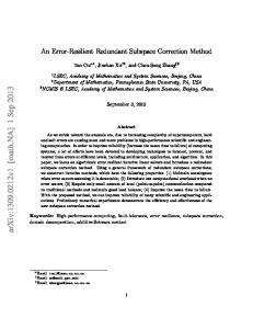
a(x) f(x) b(x) x 0

u

Figure 2.1: Theorem 2.3. and for the sake of compactness we denote

u = xk+(i?1)=J u0 = xk+i=J : We consider two quadratic functionals on V

a(x) = xT Ax ? uT Au + f (u); b(x) = xT Bx ? uT Bu + f (u); for which we have

a(u) = b(u) = f (u) and the minimum of a(x) and b(x) is attained at x = 0 (see Figure 2.1). Besides, 22

condition (2.16) implies

b(0)  f (0)  a(0) and

f (x) ? f (0)  b(x) ? b(0) for any x 2 Rn . Let u0a be a solution of the subspace problem with respect to the functional

a(x): a(u0a) = dmin a(u + di): i 2Vi We have

f (u0a) ? f (0) f (u0) ? f (0)  f (u) ? f (0) f (u) ? f (0) 0 (0)  ba((uua))??ab(0) a(u0a) ? a(0) b(u0a) ? b(0) = a(u) ? a(0)  a(u0a) ? a(0) u0 T Bu0 = i(A; u)  a0 T 0a ua Aua  i(A; u)  (A?1B ):  This theorem shows that if matrices A and B in (2.16) are close enough then the reduction of the general objective function (2.1) produced by Algorithm 2.2 can be arbitrarily close to the corresponding reduction for the quadratic objective (2.15).

23

2.2.2 Convergence Rate for Additive Schwarz Methods In this section we consider the additive Schwarz method for solving 2.1.

Alg. 2.3 - Additive Schwarz Algorithm Choose initial approximation x0 and relaxation parameters

i > 0;

J X

such that

i=1

i = 1

(2.17)

for k = 0 until convergence for i = 1 : J in parallel nd dki 2 Vi such that

f (xk + dki ) = dmin f (xk + di) i 2Vi

(2.18)

end

xk+1 = xk + PJi=1 idki end

end

Remark 2.1 The additive Schwarz method was considered by Tai and Espedal [29] with

i > 0

and

24

J X i=1

i  1:

(2.19)

In the above algorithm the condition PJi=1 i = 1 is not restrictive because if the parameters i satisfy (2.19) we can append the set of Vi by a trivial subspace

VJ +1 = 0 and choose the corresponding J +1 = 1 ? PJi=1 i.

We assume that the global error in the objective function can be bounded in terms of local gains over the subspaces. Later in this section we will give an equivalent form of this assumption that can be viewed as an analog of Assumption 1.1 (cf. [30]) for non-quadratic minimization.

Assumption 2.4 There is a constant C such that for any x 2 V there exist such vectors di 2 Vi that the following estimate holds J X  f (x) ? f (x )  C i(f (x) ? f (x + di )); i=1

(2.20)

where x is the minimizer of f (x).

Theorem 2.4 Under assumptions 2.1 and 2.4 the additive Schwarz algorithm converges and the reduction of the objective function can be characterized as

1 f (xk+1) ? f (x)  1 ? k  f (x ) ? f (x ) C; where C is given by (2.20).

Proof. The vectors dki de ned by (2.18) provide the optimal reduction in f and therefore

f (xk + dki )  f (xk + di ) 25

for any di 2 Vi. This and (2.20) imply

f (xk ) ? f (x)  C

J X i=1

i(f (xk ) ? f (x + dki )):

(2.21)

From the convexity of f (x) and the conditions on the relaxation parameters (2.17) it follows that

f (xk+1) = f xk + J X

= f



J X i=1

i=1

J X i=1

i dki

!

i(xk + dki )

!

i(f (xk + dki ))

and form (2.21) we get

f (xk ) ? f (x)  C (f (xk ) ? f (xk+1 )) or

C (f (xk+1) ? f (x))  (C ? 1)(f (xk ) ? f (x)) and

1 f (xk+1 ) ? f (x)  1 ? k  f (x ) ? f (x ) C:



As we pointed out Assumption 2.4 can be put in a dierent form. Using condition (2.17) we can perform the following chain of transformations starting

26

with (2.20)

f (x) ? f (x)  Cf (x) ? C J X

J X i=1

if (x + di)

if (x + di)  (C ? 1)f (x) + f (x) i=1 ! J X  C if (x + di ) ? f (x )  (C ? 1) (f (x) ? f (x)) C

i=1 J X i=1

i (f (x + di ) ? f (x)) 

C?1  C (f (x) ? f (x ))

and therefore Assumption 2.4 is equivalent to

Assumption 2.5 There is a constant C > 0 such that for any x 2 V there we can nd di 2 Vi such that

! 1 i (f (x + di ) ? f (x))  1 ? C (f (x) ? f (x)): i=1

J X

(2.22)

We can compare this assumption with Assumption 1.1 we mentioned in Introduction. In the case when f (x) is quadratic (2.13) the term (f (x) ? f (x)) in the right hand side of the above inequality is equal to kx ? xk2A and therefore coincides with the right hand side term of (1.10) applied to the error vector x ? x. The left hand side of (2.22) generalizes the decomposition of the error vector weighted with the relaxation parameters i.

Remark 2.2 An important distinction between our approach and the theory of Tai and Espedal [29] is that in this section we assume the convexity of f (x) in (2.1) but not its smoothness.

27

2.3 Constrained Optimization In this section we allow constraints in the problem (2.1): min f (x); x2C

(2.23)

where C  Rn is a closed convex feasible set and the function f (x) satis es the following assumption on the level surfaces of f (x).

Assumption 2.6 The sets fh = fx j f (x)  hg

(2.24)

are strictly convex for any h.

We will discuss examples of problems satisfying the assumptions of this section in Chapter 4.

Remark 2.3 Assumption 2.6 is weaker than the requirement for f to be convex, for example f (x) = kxk 21 is not convex in Rn but satis es the above assumption.

Also, as we did in the rst section of this chapter, to ensure that (2.23) has a solution we require, that f is coercive on C :

Assumption 2.7 The sets fh \ C = fx j x 2 C , f (x)  hg are bounded for all h.

28

(2.25)

The following result is straightforward.

Lemma 2.1 Under Assumptions 2.6 and 2.7 the minimization problem (2.23) has a unique solution.

Proof. First we chose h for which Ch = f h \ C is nonempty. We can replace (2.23) with an equivalent restricted problem min f (x):

x2Ch

(2.26)

As an intersection of two closed sets the set Ch is closed. Besides, the assumption that f (x) is coercive implies that Ch is bounded and therefore, since Ch 2 Rn , it is compact. That and continuity of f (x) imply that the restricted problem (2.26) has a solution. To show uniqueness we assume that x1 and x2 are solutions of (2.23):

f (x1) = f (x2) = min f (x) = H: x2C

(2.27)

Convexity of C implies that the convex combination 21 (x1 + x2) is in C , but since the set fH is strictly convex we have

x + x  f 1 2 2 < H; which violates (2.27).



We can adjust the multiplicative algorithm for the constrained problem (2.23).

29

Alg. 2.4 - Multiplicative Method for Constrained Optimization Starting with x0 2 C for k = 0 until convergence for i = 1 : J nd xk+i=J = xk+(i?1)=J + dki  C such that

f (xk+i=J ) =

min d 2V

i i xk+(i?1)=J +di C

f (xk+(i?1)=J + di)

(2.28)

end end

end

Remark 2.4 Since the restricted problem (2.28) satis es the assumptions we made for the original problem (2.23) its solution is well-de ned (Lemma 2.1).

We can formulate the theorem that under the assumptions of the above lemma the iterates generated by Algorithm 2.4 converge. Its proof is similar to the proof of Theorem 2.1.

Theorem 2.5 Under the assumptions of Lemma 2.1 Algorithm 2.4 applied to the problem (2.23) produces a convergent sequence of iterates and the limit

lim xk = x~ 2 C

k!1

30

satis es

f (~x) = min f (~x + di ); d 2V i i x~+di C

i = 1 : : :J:

(2.29)

Proof. Since all the iterates xk+i=J are contained in the compact set fx j f (x)  f (x0)g \ C they have a limit point. To show that this limit point is unique we assume the contrary. That would imply that there is a sequence of indices kj and an integer

i0  0 such that kj +(i0 ?1)=J 6= lim xkj +i0 =J = x~ : x~1 = kjlim x 2 !1 kj !1

(2.30)

kj +i0 =J ? xkj +(i0 ?1)=J ) 2 V : x~2 ? x~1 = kjlim ( x i !1

(2.31)

We have

Since the sequence f (xk+i=J ) is non-increasing we must have

f (x~1) = f (x~2) = h and since by assumption the set fx j f (x)  hg is strictly convex the midpoint satis es

! x ~ + x ~ 1 2 f 0 such that ! x~1 + x~2 f 2 +r 0;

where is a bounded region in R2 and ai;j (x) = aj;i(x), p(x)  0 are piecewise smooth real functions. To discretize the problem, we can perform a triangulation of with triangles of quasi-uniform size h and use the standard nite element approach to represent

37

(3.1) as

Ax = Mx;

(3.2)

where x is the unknown n-vector and A = AT > 0, M = M T > 0 are the stiness and the mass matrices respectively that satisfy

Assumption 3.1 The discretized stiness matrix A is an M-matrix and the mass matrix M is nonnegative componentwise.

We will also need an assumption of the irreducibility of matrices A and M which follows from

Assumption 3.2 The triangulation of that gives rise to matrices A and M forms a connected graph in R2 .

We have

Lemma 3.1 Under Assumptions 3.1 and 3.2 the smallest eigenvalue of (3.2) 1 is simple and the associated eigenvector x1 can be taken componentwise positive.

Proof. We can rewrite (3.2) as A?1Mx = ?1 x:

(3.3)

From Assumption 3.1 it follows that all the entries of A?1 and M are nonnegative and Assumption 3.2 implies that these matrices are irreducible. Therefore the product A?1M is nonnegative and irreducible. The Perron-Frobenius theorem 38

(see for example [25]) guarantees that (3.3) has a simple largest eigenvalue max and the corresponding eigenvector x1 can be chosen componentwise positive. The 1 with the same original eigenvalue problem has the smallest eigenvalue 1 = ?max

eigenvector x1

.

This lemma provides a discrete version of the corresponding result for the continuous problem (3.1) [14]. We will compute the smallest eigenvalue of (3.2) minimizing the Rayleigh quotient

xT Ax : 1 = min  ( x ) = min x6=0 x6=0 xT Mx

(3.4)

To apply the domain decomposition technique to this problem we represent

as a union of overlapping subdomains: = [Ji=1 i. Let fVi gJi=1 be the nite element subspaces corresponding to this partition and let PiT denote the orthogonal projection into the subspace Vi , its transpose Pi is the prolongation operator from

Vi to V = Rn . We also introduce the M-norm of a vector kxkM = (xT Mx)1=2. The multiplicativeSchwarz algorithm for solving (3.4) analogous to Algorithm 2.1 of Chapter 2 was proposed Kaschiev [16] and Maliassov [21]. They showed that the subspace minimization (2.2) for problem (3.4)

(xk+i=J ) = dmin (xk+(i?1)=J + Pi di) i 2Vi

(3.5)

results in an eigenvalue problem of size (ni +1)  (ni +1), where ni is the dimension of the subspace Vi . 39

To see that we introduce the notation 0 1 k BB di CCC ~dki = B @ A 1

Pik

Pi xk+ i?J1

=

(3.6)

!

(3.7)

and represent the subsequent iterate

xk+ Ji = xk+ i?J1 + Pi dki as

xk+ Ji = Pik d~ki : We can rewrite (3.5) as (Pik d~ki )T A(Pik d~ki ) di (Pik d~ki )T M (Pik d~ki ) T d~ki Aki d~ki ; = min T d~ki d~k M k d~k i i i

min (Pik d~ki ) = min ~k ~k di

(3.8)

where

Aki = Pik T APik Mik

=

Pik T MPik :

(3.9)

The form of (3.8) suggests that the subspace problem (3.5) is the eigenvalue problem with matrices Aki and Mik

Aki d~ki = (xk+ Ji )Mik d~ki : 40

(3.10)

The matrices Aki and Mik preserve the sparsity of the original matrices A and M except for the last row and column, therefore the minimization subproblem can be eciently solved by standard methods such as inverse iteration. Algorithm 2.1 of Chapter 2 applied to the eigenvalue problem (3.4) becomes

Alg. 3.1 - Multiplicative Algorithm for Eigenvalue Problem Starting with x0 for k = 0 until convergence for i = 1 : J k k using xk+(i?1)=J construct matrices 0 1 Ai and Mi and solve (3.10)

BB dki CC ~ k for min. eigenvector di = B @ CA, then update and normailize 1 xk+ Ji = xk+(i?1)=J + Pi dki xk+ Ji

xk+ Ji kxk+ Ji kM

(3.11) (3.12)

end end

end The normalization step (3.12) can be performed either after each subspace iteration or after a loop over all the subspaces is completed. The convergence of this algorithm was proven in [16] and [21] with the assumption that the initial

41

guess x0 satis es

1 < (x0) < 2:

(3.13)

Lui [20] pointed out that the algorithm can break down in certain degenerate cases when it faces the problem of not being able to nd the required correction from a current subspace (3.5). This happens when the solution to the eigenvalue problem (3.10) has a zero component corresponding to the previous iterate 0 1 0 1 B dk C B dki CC (3.14) Aki B B@ CA = (xk+ Ji )Mik BB@ i CCA 0 0 and therefore cannot be scaled to match (3.6). Lui proved convergence to the smallest eigenvalue 1 for a modi ed algorithm in the case of two subdomains under condition (3.13). Before we proceed we formulate a lemma that guarantees that once initialized with a componentwise positive vector the iterates produced by Algorithm 3.1 cannot have components of mixed signs.

Lemma 3.2 Under Assumptions 3.1 and 3.2 if Algorithm 3.1 is initialized with a componentwise positive x0 and if the subsequent iterates xk+ Ji are de ned, they are also componentwise positive.

Proof. We will argue by contradiction. Suppose x is the rst iterate of Algorithm 3.1 that has a non-positive component. First we assume 0 that1x does not have zero B xp CC CA ; where components components and therefore can be represented as x = B B@ ?xn 42

of xp and xn are positive. Let 1 0 B App Apn CC CA A=B B @ T Apn Ann

1 0 B Mpp Mpn CC CA M =B B@ MpnT Mnn

0 1 B xp C C B@ C be the corresponding partitionings of A and M . For the vector x+ = B A we xn have xT+Ax+ = xTp Appxp + 2xTp Apnxn + xTn Annxn < xTp Appxp ? 2xTp Apnxn + xTn Annxn = xT Ax: The inequality is strict because Assumption 3.2 implies that A and M are not block diagonal and therefore the block Apn cannot be zero. Similarly

xT+ Mx+ > xT Mx and

(x+ ) < (x): Since we assumed that x is produced from a positive vector by changing some of its components we conclude that x+ can be formed the same way and therefore x cannot correspond to the optimal choice of the subspace correction. If x has zero components then for x+ that is again formed of the absolute values of the components of x the above inequalities are not necessarily strict

(x+ )  (x): 43

In this case the representation of x+ is

0 1 B xp CC x+ = B B@ CA ; x0

(3.15)

where xp > 0 and x0 is a zero block. Then the vector 1 0 CC B xp CA ; x~+ = B B@ ? 1 ?A00 ATp0xp where A00 and Ap0 are the blocks of A corresponding to the partition (3.15), is componentwise positive. We have

x~T+ Ax~+ = xT+ Ax+ ? xTp Ap0A?001ATp0xp < xT+ Ax+

 xT Ax and

x~T+M x~+ > xT+ Mx+

 xT Mx: For the same reasons as above the vector x cannot result from the optimal subspace correction of a positive vector because the vector x~+ can be produced by a correction from the same subspace and results in a greater reduction of .



The breakdown of the algorithm (3.14) occurs if the eigenvector corresponding to the minimum eigenvalue is contained in one of the subspaces Vi . To prevent 44

this we can formulate a natural assumption that this eigenvector is not contained in any of the subspaces Vi , which means that the Rayleigh Quotient over each of the subspaces Vi should exceed the minimum eigenvalue 1 .

Assumption 3.3 For all subspaces Vi the constants dTi PiT APidi (1i)  dmin  ( d ) = min i di 2Vi dT P T MP d i 2Vi i i

i i

(3.16)

satisfy (1i) > 1.

Lemma 3.3 Let Assumptions 3.1, 3.2 and 3.3 hold and let Algorithm 3.1 be initialized with a componentwise positive vector x0. Then for all i and k the eigenvector d~ki corresponding to the lowest eigenvalue of (3.10) has a nonzero last component and therefore the update step (3.11) of Algorithm 3.1 is well-de ned.

Proof. Assuming the contrary we can rewrite (3.14) using (3.7) and (3.9) as PiT APidki = (Pi dki )PiT MPi dki xk+(i?1)=J T (APidki ? (Pi dki )MPi dki ) = 0:

(3.17)

From the rst condition it follows that ((Pi di); di) is the lowest eigenpair of the problem with matrices PiT APi and PiT MPi : These matrices satisfy Assumption 3.1, and because of Lemma 3.1 the eigenvector dki can be taken componentwise positive. The residual vector

rik = APidki ? (Pi dki )MPi dki 45

satis es Pi?rik  0 componentwise since, as an M-matrix, A has non-positive odiagonal block Pi? APi and the corresponding block of M is nonnegative. Besides,

Pi rik = 0 and therefore, rik  0 componentwise. Since xk+(i?1)=J is componentwise positive (Lemma 3.2) from (3.17) it follows that rik = 0 which in turn implies that Pidi is an eigenvector of the unrestricted problem (3.2). Since Pi di has all its components of the same sign we have (Pidi ) = 1 which violates Assumption 3.3.



This lemma shows that the subspace correction update (3.11) is always wellde ned. Now we can formulate the convergence result.

Theorem 3.1 Let Assumptions 3.1, 3.2 and 3.3 hold then vectors xk and the corresponding Rayleigh quotients (xk ) produced by Algorithm 3.1 converge to the lowest eigenpair of discretized problem (3.2) if x0 is chosen componentwise positive.

Proof. Since the sequence (xk+i=J ) is non-increasing and bounded from below by 1 it converges. We will show that its limit ~ is an eigenvalue of (3.2) and that the sequence xk converges to the corresponding eigenvector x~. Then using Lemmas 3.1 and 3.2 we will show that ~ = 1. First we point out that for any k and i we have

(xk+ Ji ) < (1i);

(3.18)

where (1i) is given by (3.16). To show that we notice that choosing x = Pdi, where di is the optimal vector for (3.16) we have (x) = (1i) but, as it follows from 46

Lemma 3.3, the optimal xk+ Ji is of the form xk+ i?J 1 + Pidki and since the lowest eigenvalue of the restricted problem is simple we have (3.18). From (3.10) it follows that

    PiT A ? (xk+ Ji )M Pi dki = PiT (xk+ Ji )M ? A xk+ i?J1

(3.19)

and

   T T xk+ i?J1 A ? (xk+ Ji )M Pidki = xk+ i?J1 Mxk+ i?J1 (xk+ Ji ) ? (xk+ i?J1 ) : Combining the two equations above we get

    T dki T PiT A ? (xk+ Ji )M Pi dki = xk+ i?J1 Mxk+ i?J1 (xk+ i?J1 ) ? (xk+ Ji ) : (3.20) Since (xk+i=J ) converges as k ! 1 and because of normalization (3.12) the right hand side of the above expression converges to zero as k ! 1 for every i therefore the left hand side converges to zero. Using (3.18) and (3.16) we can estimate the left hand side of (3.20)

  dki T PiT (A ? (xk+ Ji )M )Pi dki > (1i) ? (xk+ Ji ) dki T PiT MPi dki    (1i) ? (x0+ Ji ) dki T PiT MPi dki > dki T PiT MPi dki ; where

 J  (i) 0+ Ji ) > 0  = min  ?  ( x 1 i=1 47

and since the left hand side of (3.20) converges to zero and M is positive de nite we conclude that the vectors Pidki converge to zero componentwise as k ! 1 for every i and the iterates xk+i=J converge to an M -normalized limit x~. If we take the limit of (3.19) we get

PiT (~M ? A)~x = 0 and since the prolongation operators Pi span the entire space we have (A ? ~M )~x = 0 which shows that (~; x~) is an eigenpair of (3.2). From Lemma 3.2 it follows that

x~ is componentwise positive and since the eigenvectors are M -orthogonal and the smallest eigenvalue is simple and the corresponding eigenvector is componentwise positive we conclude that (~; x~) is the lowest eigenmode of (3.2).



3.1.2 Coarse Grid Correction and Multilevel Method We can modify Algorithm 3.1 to include the coarse grid correction after a loop over the subdomains is completed as we did for Algorithm 2.2. The eect of the this correction for a model problem of 2-D Laplacian in a unit square is shown in Figures 3.1 and 3.2. We can see that without the coarse grid the convergence rate is dependent on both the meshsize and the number of subdomains whereas after the coarse grid correction has been added the convergence rate becomes independent of both ne and coarse meshsizes h and H . 48

h=1/12; H=1/4,1/6

2

10

0

0

10

10

−2

−2

10 Error

Error

10

−4

10

−6

−4

10

−6

10

10

−8

−8

10

10

−10

10

0

−10

2

4 Iterations

6

10

8

h=1/24; H=1/4,1/6,1/8,1/12

2

2

4 Iterations

6

8

h=1/32; H=1/4,1/8,1/16

10

0

2

10

10

−2

0

10 Error

10 Error

0 4

10

−4

10

−6

−2

10

−4

10

10

−8

−6

10

10

−10

10

h=1/16; H=1/4,1/8

2

10

0

−8

2

4 Iterations

6

10

8

0

2

4 Iterations

6

8

Figure 3.1: Algorithm 3.1 for 2D Laplacian without the coarse grid correction.

49

h=1/12; H=1/4,1/6

5

10

0

0

10 Error

Error

10

−5

10

−10

10

−15

0

−5

10

−10

10 10

h=1/16; H=1/4,1/8

5

10

−15

2

4

10

6

0

2

Iterations h=1/24; H=1/4,1/6,1/8,1/12

5

4

6

Iterations h=1/32; H=1/4,1/8,1/16

5

10

10

0

10

0

Error

Error

10 −5

10

−5

10

−10

10

−15

10

0

−10

2

4

10

6

Iterations

0

1

2 Iterations

3

4

Figure 3.2: Algorithm 3.1 for 2D Laplacian with the coarse grid correction.

50

Since the subspace problem is of the same type as the original one i.e. a generalized eigenvalue problem, we can make the algorithm more ecient by applying it recursively. Instead of solving the eigenvalue subproblem over a subdomain by some other method we can apply several iterations of the same algorithm. Applying that recursion to the multiplicative method with coarse grid correction we can view the resulting scheme as a multilevel method and the iterations performed on each level as the smoothing of the solution. As we pointed out in section 2.4, the recursion can be stopped once the subproblems we are solving reached some small enough xed size Cc and traditional inverse iteration can be applied. We should remark that at each successive level the subproblem matrices get appended by a dense row and column. We may think of the corresponding component as of a ctitious gridpoint for a subdomain at the current level. At the coarsest level the subproblem matrices will be appended by rows and columns coming from the previous levels. Though the presented algorithms are sequential we can add some degree of parallelism using multicoloring technique (see for example [8]).

3.1.3 Alternative Variational Characterization of the Smallest Eigenvalue A dierent variational formulation for the symmetric positive de nite eigenvalue problem (3.2) was described by Mathew and Reddy (94) [23]. They pointed 51

out that the minimal eigenpair (x1, 1) can be characterized as: T T 2 (x1) = min x  (x)  min x (x Ax + (1 ? x Mx) )

with

(3.21)

q 1 = 2 ? 42 ? 4(x1)

and

kx1k2M = 1 ? 21

(3.22)

 > 1=2:

(3.23)

for any

Unlike the Rayleigh Quotient minimization, formulation (3.21) is unconstrained. The -term in (x) serves as a barrier to pull x away from the trivial solution 0. Using

!

Pik = Pi xk+(i?1)=J 0 1 BB dki CC ~ k di = B @ k CA ; i we can write the minimizaition step (2.2) of the multiplicative algorithm as (xk+i=J ) = dimin J (Pik d~i ) 2Vi ; i h k~ T k~ k d~i )T M (P k d~i ))2 = min d ) +  (1 ? ( P ( P d ) A ( P i i i i i i d~i   T = min d~i Aki d~i + (1 ? d~iT Mik d~i )2 ~ di

52

with

Aki = Pik T APik Mik = Pik T MPik : We can see that the subspace problem is again of the same type as the original problem (3.21). To make it the eigenvalue problem with matrices (Aki ; Mik ) we should make a restriction on  similar to (3.23) replacing 1 by the current value of the Rayleigh quotient (xk+i=J ). Since the sequence of the Rayleigh Quotients is non-increasing we can choose  satisfying

 > (x0)=2 = 0=2:

(3.24)

Similarly condition (3.22) becomes

kxk+i=J k2M = 1 ? (xk2+i=J )  1?

(x0 ) : 2

(3.25)

Remark 3.1 For any choice of  satisfying (3.24), one subspace correction step for formulations (3.4) and (3.21) results in the same reduced generalized eigenvalue problem with matrices (3.9). The application of the multiplicative Schwarz algorithm to both formulations results in the same approximations to the lowest eigenvalue and the approximations to the eigenvector are the same up to normalization.

The following lemma estimates the Hessian matrix of (x)

H (x)  r2(x) = 2(A ? 2M ) + 8M (xxT )M + 4(xT Mx)M: 53

(3.26)

in terms of A near the solution of (3.21). This estimate will allow us to use the theory of Multiplicative Schwarz methods for minimization problems developed by Tai and Espedal [29].

Lemma 3.4 Let 1 + 2 2

(3.27)

 1 ? 20  kxk2M  1:

(3.28)

(x)  0 < and

Then if  = 43 0 the Hessian (3.26) satis es

c1A < H (x) < c2A;

(3.29)

where the constants c1 and c2 can be chosen independently of the discretization parameters.

Remark 3.2 Conditions (3.27) and (3.28) provide the directional and the radial restrictions on x. The equivalence of the minimization of (x) and (x) (Remark 3.1) implies that that if condition (3.27) is satis ed for the initial approximation

x0 it is satis ed for all the subsequent iterates xk . The radial estimate (3.28) is not restrictive because even if it is not satis ed by x0 condition (3.25) enforces it for all the subsequent iterates.

Proof. Given x satisfying (3.27) and (3.28) we can represent any y 2 Rn as y = y x + y? ; 54

where yx is the M -orthogonal projection of y on span(x). Condition (3.27) implies that there is  2 (0; 21 ) such that

(x) < 0 = (1 ? )1 + 2

(3.30)

and since y? is M -orthogonal to x we have

(y? )  1 + (1 ? )2:

(3.31)

Using the lower bound for kxk2M from (3.28) we get

y?T Hy?

! 0  + 4(1 ? 2 )M y? = y?T (2(A ? 0M ) + 8M (xxT )M ) y? y?T

2(A ? 2M ) + 8M (xxT )M

 2(y?T Ay? ? 0y?T My? )

! 0 T = 2 1? (y? ) y?Ay?  2 (1 ? 2)(+2 ? 1) y?T Ay?; 1 2

(3.32)

where the last inequality follows from (3.30) and (3.31). We also have

y?T Hyx = 2y?T Ayx

(3.33)

and with our chose of  = 43 0

yxT Hyx  2(yxT Ayx ? 0yxT Myx) + 8(xT Mx)(yxT Myx) ! 0 T T T  2(yx Ayx ? 0yx Myx) + 8 1 ? 2 (yx Myx) = 2(yxT Ayx + (4 ? 30)yxT Myx) = 2yxT Ayx:

(3.34) 55

Since for  2 (0; 21 ) 2

(1 ? 2)(2 ? 1) 11

(4.18)

then  = 0 and b that solves (4.14) also solves

  T b)2 + 2ka ? B bk2 : min (  ? b 11 21 2 2 b

(4.19)

Since the objective function in (4.19) is smooth, its gradient should be equal to zero at the solution 4(bT b ? 11)b + 4(B2T B2b ? B2T a21) = 0 or ((bT b ? 11)I + B2T B2)b = B2T a21:

(4.20)

This problem can be solved using the Newton's method. For   0 we consider

b = (I + B2T B2)?1B2T a21 82

(4.21)

1.5 1 0.5

f(sigma)

0 −0.5 −1 −1.5 −2 −2.5 −3 0

0.2

0.4

0.6

0.8

1 sigma

1.2

1.4

1.6

1.8

2

Figure 4.2: Monotonicity of f () for the factor analysis problem. and

f () = bT b ? 11 ? :

(4.22)

It is easy to see that if f () = 0 then the corresponding b solves (4.20). This solution exists because (4.18) implies f (0) > 0 and lim!+1 = ?1. Uniqueness follows from the monotonicity of f () that is shown below. From (4.21) we obtain

@b T ?1 @ = ?(I + B2 B2) b

83

and therefore

@f T @b ? 1 = 2 b  @ @ = ?2bT (I + B2T B2)?1b ? 1 < 0: A typical example of f () is shown on Figure 4.2. We can apply the Newton's method for solving f (b()) = 0:

Alg. 4.3 - Newton's Method for solving (4.21), (4.22) Initialize  (say  = 0) Compute b by (4.21) Compute f () and

@f () @

from (4.22) and (4.23).

Update  using Newton's step 

 ? f ()( @f@() )?1

Repeat the Newton's procedure

end The entire procedure for solving the problem (4.11) becomes:

84

(4.23)

Alg. 4.4 - Block Gauss-Seidel method. Factor Analysis Problem Initialize M 0 = B 0 B 0T and D0 = diag(d0 )2 for k = 0 until convergence for i = 1 : n Update i-th row of B k+(i?1)=n and  = dik+(i?1)=n solving (4.14) either by (4.16)-(4.17) or using Newton's Method to get B k+i=n and dk+i=n . Update the iterates:

M k+i=n = B k+i=nB k+i=n T

D = diag(dk+i=n )2

end end

end The reduction in the objective function for problems of sizes 20  20 and 40  40 are shown in Figure 4.3.

4.3 Gain-Loss Optimization

85

20 by 20 problem

2

10

1

10

0

10

−1

Error

10

−2

10

−3

10

−4

10

−5

10

0

5

10

15

10

15

Iterations 40 by 40 problem

3

10

2

10

1

10

0

Error

10

−1

10

−2

10

−3

10

−4

10

−5

10

0

5 Iterations

Figure 4.3: Error reduction for the factor analysis problem with n = 20 and n = 40.

86

4.3.1 Problem Formulation The gain-loss optimization constitutes an alternative to the mean-variance optimization for portfolio selection [22]. Let B be an n  m matrix B each of whose columns contain returns for a particular stock and whose rows correspond to dierent times when this returns are computed. For any m-vector x whose components represent the weights of the stocks in a portfolio the components of the product

ri = (Bx)i give the returns for the portfolio at dierent times. The positive part ri+ and the negative part ri? of the return components correspond to the gain and the loss respectively. We consider the gain-loss optimization problem of nding a portfolio x that minimizes the loss Pm r? while the gain Pm r+ is kept xed. i=1 i

i=1 i

Because of the relations

ri+ ? ri? = (Bx)i ri+ + ri?

= j(Bx)ij

(4.24)

and consequently

ri+ = ri? =

j(Bx)ij + (Bx)i 2

j(Bx)ij ? (Bx)i 2

the gain-loss optimization problem can be put in an equivalent form of minimizing the sum of the gain and the loss min x f (x) = min x kBxk1 87

(4.25)

subject to the overall return Pmi=1 ri being held xed n X (Bx)i = : i=1

(4.26)

We assume that the portfolio x is normalized, i.e. the weights (which can be negative) add up to one m X j =1

(x)j = 1:

(4.27)

Remark 4.3 To avoid multiple solutions of the problem (4.25)-(4.27) we assume that the dimensions of B satisfy m < n + 2 and that the columns of B are linearly independent. For many practical problems we have m  n.

In order to allow the future derivation of the block Gauss-Seidel method for this problem we generalize the objective function (4.25) min x F (x) = min x kBx ? f k1 ;

(4.28)

where f is a given n-vector. We will also normalize the condition (4.26) replacing

B by B : n X i=1

(Bx)i = 1:

(4.29)

Introducing an m-vector e of ones and an m-vector bc of column-sums of B we can represent the constrains (4.27) and (4.29) as

eT x = 1

and 88

bTc x = 1:

(4.30)

The problem (4.28), (4.30) can be transformed to a linear programming formulation (cf. [10]). Representing the residual vector as a dierence of two vectors with nonnegative components (Bx ? f )i = ri+ ? ri? we can formulate the equivalent problem as min x;r

n X i=1

! n X ri+ + ri? i=1

Subject to

Bx +r+ ? r? = f eT x

= 1

bTc x

= 1

r  0 Several algorithms based on the simplex method were proposed for this problem ([2], [3]), but in this work we will apply an interior point method analogous to the one discussed in [31]. We can represent x as xj = x+j ? x?j and put the problem in canonical form ! n n X X ? + (4.31) ri + ri ; min x ;r i=1

i=1

subject to

Bx+ ? Bx? +r+ ? r? = f eT x+ ? eT x?

= 1

bTc x+ ? bTc x?

= 1

xj ; ri

 0:

89

(4.32)

The matrix of the constraints for this problem is 0 BB B ?B I ?I BB Ap = B BB eT ?eT 0 0 B@ bTc ?bTc 0 0

1 CC CC CC : CC A

4.3.2 Dual Problem and Interior Point Algorithm The dual for the problem (4.31), (4.32) is max f T y +  +

y2Rn ;;

subject to

0 0 1 BB 0m BB y CC BB BB CC BB 0m B ATp B BB  CCC  BB B@ CA BB en BB @ en

1 CC CC CC CC ; CC CC CA

which can be written as min ?f T y ?  ?

y2Rn ;;

with

B T y + eT  + bTc = 0n

?1  yj  1

j = 1 : : : n:

Changing

yj + 1 ! yj 90

(4.33)

and adding slack variables zj , j = 1 : : : n we get the problem in canonical form. min ?f T y ? + ? + + ? + ?

y;z; ; 

subject to

B T y + eT + + bTc + ? eT ? ? bTc ? = bc yj + zj = 2

j = 1:::n

yj ; zj ; ;   0 The constraint matrix of this problem is 1 0 T B B C 0 CC CA ; Ad = B B@ I 0 I where the block C is given by ! C = e bc ?e ?bc :

(4.34)

(4.35)

We can rewrite this problem in a more compact form min c~T y~ y~

(4.36)

subject to

Ady~ = ~b; where

0 1 BB y CC BB CC y~ = B BB a CCC ; B@ CA z

0 BB + BB BB + BB a=B BB ? BB @ ?

y~  0;

1 CC CC 0 CC CC ; ~b = BBB bc CC @ 2en CC CA

91

0 1 BB ?f BB CC CA ; c~ = BB c BB @ 0n

(4.37)

1 CC CC CC ; CC A

0 BB ?1 BB BB 1 BB c=B BB ?1 BB @ 1

1 CC CC CC CC : CC CC CA

Since this problem is equivalent to the dual of of (4.25)-(4.26), its dual is quivalent to the original problem and it is easy to verify that the solution to the dual of (4.36)-(4.37) is

0 1 B x CC x~ = ? B B@ CA : r+ To recover the solution x of the original problem (4.28), (4.30), we can apply

the iterior point algorithm (see for example [1] p.84) to (4.25)-(4.26):

92

Alg. 4.5 - Interior Point Algorithm for solving LP-problem (4.36)-(4.37) 1. Set k = 0, start with a feasible interior y~0 (i.e. Ady~0 = ~b, y~0 > 0) 2. De ne

D = Dk = diag(y1k ; y2k; : : :ynk ) 0 1 k B x CC 3. Find the primal estimate x~k = ? B B@ CA by solving k r+ (AdD2 ATd )~xk = AdD2c~

(4.38)

4. Find z k = c~ ? ATd x~k and the step direction

dy~k = ?D2 zk 5. Update the dual estimate by

y~k+1 = y~k + dy~k ; where 0 <  < 1 # " k y ~i : for dy~k > 0 ? dy~k  = min i i

and

i

6. Terminate if stopping criteria are satis ed, otherwise go to 2.

end

93

Remark 4.4 The structure of (4.36)-(4.37) allows to initialize the method with a (2n + 4)-vector of ones

y~0 = e2n+4 which is feasible for this problem.

The only computationally involved stage of Algorithm 4.5 is step 3 which requires forming the matrix AdD2 ATd and solving a linear system (4.38) with it. The advantage of the dual formulation described in this section is that for the matrix

Ad given by (4.34) we have

0 BB B T Dy2B + CDa2C T Dy2 B T 2 T AdD Ad = B @ Dy2 + Dz2 BDy2

1 CC CA ;

where Dy ; Dz are the blocks of D corresponding to y; z variables and Da to ; respectively. Since this matrix has a big diagonal block Dy2 + Dz2 we can use its Schur complement

S = B (Dy2 ? Dy2 (Dy2 + Dz2 )?1Dy2)B T + CDa2C T

(4.39)

to compute the action of its inverse. The matrix (4.39) is easily computable and the cost of computation for a dense matrix B is O(nm2). Direct computation of the inverse of S which is of the size

m  m requires O(m3) < O(nm2) operations. Therefore, we can conclude that the cost one iteration of the algorithm is O(mn2). This makes it more advantageous to use the dual formulation of the linear programming problem with the matrix 94

of constraints Ad (4.34) rather than the primal one with the matrix Ap (4.33) whose structure doesn't allow to use fewer than O(n3) operations per iteration when applying the interior point iteration.

4.3.3 Subspace Correction and Gauss-Seidel Method As we did in previous sections we can apply the subspace correction approach to the problem (4.28), (4.30). Let x be the current feasible approximation to the solution and P be an m  ni prolongation matrix (ni < m). The best correction

x

x + Pd, where d is a ni -vector satis es min kBPd + Bx ? f k1

d2Rk

(4.40)

subject to m X i=1

(BPd)i = 1 ?

m X i=1

(Bx)i = 0

(4.41)

and n X j =1

(d)j =

n X j =1

(Pd)j = 1 ?

n X j =1

(x)j = 0:

(4.42)

The problem (4.40)-(4.42) is of the same type as (4.28), (4.30) and therefore

95

can be solved by the same interior point procedure with the following adjustments:

x ! d B ! BP

(4.43)

C ! CP

(4.44)

f ! f ? Bx c ! 04 : We can see that because of (4.43) and (4.44) the Schur complement (4.39) for the subspace problem is related to the original one as

S ! PSP T : Therefore, performing one iteration of the interior point algorithm applied to a subspace problem corresponds to performing one step of the Gauss-Seidel method for the linear problem (4.38) of Algorithm 4.5 applied directly to (4.36)-(4.37). As we pointed out in Section 2.3, Algorithm 2.4 can converge to a boundary point of the feasible set which is not the solution of the problem but further improvement over the subspaces Vi is not possible. This situation is illustrated in Figure 4.4. We consider two examples with matrices B of sizes 128  32 and 1000  10 that contain actual stock data. In both cases we represent the unknown variables as three overlapping groups and apply Algorithm 2.4 to the corresponding problems (4.28), (4.30) using one iteration of Algorithm 4.5 to approximate the solution of the subspace problems. From 96

the plots we can see that if we choose the value of the parameter  in step 5 of Algorithm 4.5 large the iterates converge to a point that does not optimize the objective function. To explain this we should point out that the parameter  < 1 controls the rate with which the iterates approach the boundary of the feasible region. Small values of  postpone hitting the boundary at the point where further improvement in the objective along the chosen subspaces is not possible. Nevertheless, the subspace correction method that produces the iterates that converge to the true solution can still be applied to (4.28), (4.30). Rather than using Algorithm 4.5 as a method for solving the subspace problems of Algorithm 2.4 we can use it directly to solve (4.28), (4.30) but apply the subspace correction method (in this case Gauss-Seidel) to its crucial step (4.38). We conclude this chapter illustrating the solution of (4.25)-(4.27) for dierent values of  and generating the ecient frontier shown in Figure 4.5. The point on the frontier that maximizes the ratio Pn (Bx) i i=1 kBxk1 can be found by solving (4.25) using just one normalization constraint (4.27). Finally, the ecient frontier in terms of gain-loss variables Pm r+ and Pm r? i=1 i

can be found using the transformation (4.24) and is shown in Figure 4.6.

97

i=1 i

128 by 32

0.75 0.55 0.35 0.15 −3

Error

10

−4

10

0

2

4

6 Iterations

8

10

12

1000 by 10

0.75 0.55 0.35 0.15

Error

−3

10

−4

10

0

2

4

6 Iterations

8

10

12

Figure 4.4: Error reduction for the l1-norm minimization problem with 3 subdomains and dierent values of .

98

128 by 32

2

sum(B*x)

1.5

1

0.5

Tangency portfolio

0

Multiples of Tangency portfolio Efficient Frontier

−0.5 0

0.5

1

1.5

2 2.5 sum(abs(B*x))

3

3.5

4

1000 by 10

1.8

Tangency portfolio Multiples of Tangency portfolio

1.6

Efficient Frontier

1.4

sum(B*x)

1.2 1 0.8 0.6 0.4 0.2 0 −0.2 0

2

4

6 sum(abs(B*x))

8

10

12

Figure 4.5: Ecient frontier for the minimization of the l1-norm.

99

128 by 32 3

2

1.5

1

Tangency Portfolio

0.5

Multiples of Tangency Portfolio Gain−Loss Efficient Frontier

0 0

0.2

0.4

0.6

0.8 1 1.2 Loss = neg(sum(B*x))

1.4

1.6

1.8

2

1000 by 10 6

5

Gain = pos(sum(B*x))

Gain = pos(sum(B*x))

2.5

4

3

2

Tangency Portfolio

1

Multiples of Tangency Portfolio Gain−Loss Efficient Frontier

0 0

1

2

3 4 Loss = neg(sum(B*x))

5

Figure 4.6: Gain-loss ecient frontier.

100

6

Bibliography

[1] A. Arbel. Exploring Interior-Point Linear Programming. MIT Press, 1993. [2] R.D. Armstrong and J.P. Godfrey. Two linear programming algorithms for the discrete l1 norm problem. Mathematics of Computation, 33:289{300, 1979. [3] I. Barrodale and F.D.K. Roberts. An improved algorithm for discrete l1 linear approximation. SIAM J. Numer. Anal., 10:839{848, 1973. [4] T.J. Barth. SIMPLEX2D user guide. Available at http://oldwww.nas.nasa.gov/~barth/c++/guide.ps.Z, 1995. [5] F. Bourquin and F. Hennezel. Application of domain decomposition techniques to modal synthesis for eigenvalue problems. In Fifth International Symposium on Domain Decomposition Methods for Partial Dierential Equations (Norfolk, VA, 1991), pages 214{223, Philadelphia, 1992. SIAM.

[6] J.H. Bramble, J.E. Pasciak, J. Wang, and J. Xu. Convergence estimates for product iterative methods with applications to domain decomposition. Math. Comp., 57(195):1{21, 1991.

101

[7] T.F. Chan, S. Go, and L. Zikatanov. Lecture notes on multilevel methods for elliptic problems on unstructured grids. Technical Report (CAM) 97-11, Department of Mathematics, University of California, Los Angeles, CA 900951555, 1997. [8] T.F. Chan and T.P. Mathew. Domain decomposition algorithms. In Acta Numerica, pages 61{143. Cambridge Univ. Press, Cambridge, 1994.

[9] T.F. Chan and W.K. Szeto. On the optimality of the median cut spectral bisection graph partitioning method. SIAM J. Sci. Comput., 18(3):943{948, 1997. [10] A. Charnes, W.W. Cooper, and R. Ferguson. Optimal estimation of executive compensation by linear programming. Management Science, 2:138{151, 1955. [11] D.K. Fadeev and V.N. Fadeeva. Computational Methods of Linear Algebra. W.H. Freeman and Company, San Francisco, 1963. [12] C. Farhat and M. Geradin. On a component mode synthesis method and its application to incompatible substructures. Computers and Structures, 51:459{ 473, 1994. [13] E. Gelman and J. Mandel. On multilevel iterative methods for optimization problems. Math. Progr., 48:1{17, 1990.

102

[14] D. Gilbarg and N.S. Trudinger. Elliptic Partial Dierential Equations of Second Order. Springer-Verlag, 1983.

[15] W. Hackbusch. Multigrid Methods. Springer-Verlag, 1984. [16] M.S. Kaschiev. An iterative method for minimization of the Rayleigh-Ritz functional. In Computational processes and systems, No. 6 (Russian), pages 160{170. Nauka, Moscow, 1988. [17] O. Ledoit and P. Santa-Clara. Estimating large conditional covariance matrices with an application to risk management. Technical report, The Anderson School at UCLA, 1997. [18] P.L. Lions. On the schwarz alternating method. i. In First International Symposium on Domain Decomposition Methods for Partial Dierential Equations,

pages 1{42, Philadelphia, 1988. SIAM. [19] S.H. Lui. Domain decomposition for eigenvalue problems (preprint). Hong Kong Univ. of Science and Tech., 1995. [20] S.H. Lui. On two Schwarz alternating methods for the symmetric eigenvalue problem (preprint). Hong Kong Univ. of Science and Tech., 1996. [21] S.Yu. Maliassov. On the analog of Schwarz method for spectral problems. In Numerical methods and mathematical modeling (Russian), pages 70{79. Otdel

Vychisl. Mat., Moscow, 1992.

103

[22] H.M. Markowitz. Portfolio selection. Journal of Finance, 7(1):77{91, 1952. [23] G. Mathew and V.U. Reddy. Development and analysis of a neural network approach to Pisarenko's harmonic retrieval method. IEEE Trans. Sig. Proc., 42(3):663 { 673, 1994. [24] S.F. McCormick. Multilevel Projection Methods for Partial Dierential Equations. SIAM, Philadelphia, 1992.

[25] J.M. Ortega. Matrix Theory. Plenum Press, New York, 1987. [26] B.N. Parlett. The Symmetric Eigenvalue Problem. Prentice-Hall, Inc., Englewood Clis, NJ, 1980. [27] L. Rudin, S. Osher, and E. Fatemi. Nonlinear total variation based noise removal algorithms. Physica D, 60:449{458, 1992. [28] A. Stathopoulos, Y. Saad, and C.F. Fischer. A Schur complement method for eigenvalue problems. In Proceedings of the Seventh Copper Mountain Conference on Multigrid Methods, April 2-7 1995.

[29] X.-C. Tai and M. Espedal. Rate of convergence of some space decomposition methods for linear and nonlinear problems. SIAM J. Numer. Anal. (to appear), 1997.

[30] J. Xu. Iterative methods by space decomposition and subspace correction. SIAM Rev., 34:581{613, 1992.

104

[31] Y. Zhang. Primal-dual interior point approach for computing l1-solutions and

l1-solutions of overdetermined linear systems. J. of Optim. Theor. and Appl., 77(2):323{341, 1993.

105