Multiple Quantitative Trait Loci Mapping With ... - Semantic Scholar

Copyright  2004 by the Genetics Society of America DOI: 10.1534/genetics.104.030296

Multiple Quantitative Trait Loci Mapping With Cofactors and Application of Alternative Variants of the False Discovery Rate in an Enlarged Granddaughter Design Jo¨rn Bennewitz,*,1 Norbert Reinsch,† Volker Guiard,† Sebastien Fritz,‡ Hauke Thomsen,§ Christian Looft,* Christa Ku¨hn,† Manfred Schwerin,† Christina Weimann,** Georg Erhardt,** Fritz Reinhardt,§ Reinhard Reents,§ Didier Boichard†† and Ernst Kalm* *Institute of Animal Breeding and Husbandry, University of Kiel, D-24098 Kiel, Germany, †Research Institute for the Biology of Farm Animals, D-18196 Dummerstorf, Germany, ‡UNCEIA, 75595 Paris 12, France, §United Datasystems for Animal Production (VIT), D-27283 Verden/Aller, Germany, ††Station de Ge´ne´tique Quantitative et Applique´e, INRA, 78352 Jouy en Josas, France and **Institute of Animal Breeding and Genetics, University Giessen, D-35390 Giessen, Germany Manuscript received April 21, 2004 Accepted for publication June 10, 2004 ABSTRACT The experimental power of a granddaughter design to detect quantitative trait loci (QTL) in dairy cattle is often limited by the availability of progeny-tested sires, by the ignoring of already identified QTL in the statistical analysis, and by the application of stringent experimentwise significance levels. This study describes an experiment that addressed these points. A large granddaughter design was set up that included sires from two countries (Germany and France), resulting in almost 2000 sires. The animals were genotyped for markers on nine different chromosomes. The QTL analysis was done for six traits separately using a multimarker regression that included putative QTL on other chromosomes as cofactors in the model. Different variants of the false discovery rate (FDR) were applied. Two of them accounted for the proportion of truly null hypotheses, which were estimated to be 0.28 and 0.3, respectively, and were therefore tailored to the experiment. A total of 25 QTL could be mapped when cofactors were included in the model—7 more than without cofactors. Controlling the FDR at 0.05 revealed 31 QTL for the two FDR methods that accounted for the proportion of truly null hypotheses. The relatively high power of this study can be attributed to the size of the experiment, to the QTL analysis with cofactors, and to the application of an appropriate FDR.

M

UCH effort has been undertaken to identify quantitative trait loci (QTL) associated with genetic variation for traits of economic or scientific interest in livestock species with the aid of genetic markers. Hayes and Goddard (2001) estimated the number of QTL in dairy cattle for a trait that undergoes selection at about 50 to 100 depending on the size of the effective population. With regard to this, the majority of QTL remained undetected by the experiments undertaken so far. The main reason for this is that the distribution of the QTL effects follow likely a gamma distribution with many QTL of small effects and only a few of large effects (Hayes and Goddard 2001) and that QTL experiments conducted to date are not powerful enough to detect the QTL of smaller effects. In QTL mapping in pigs it is common to generate an F2 cross of different, ideally divergent selected, breeds. As generating such a cross in dairy cattle is a timeconsuming and costly process, most dairy cattle QTL

1 Corresponding author: Institute of Animal Breeding and Husbandry, University of Kiel, D-24098 Kiel, Germany. E-mail: [email protected]

Genetics 168: 1019–1027 (October 2004)

experiments used the existing male half-sib structure by setting up the so-called granddaughter design (Weller et al. 1990). In this design the pedigree consists of sets of genotyped and progeny-tested male half-sib families. The power to detect QTL in a granddaughter design is largely influenced by the size of the half-sib families, which has its limit in the availability of progeny-tested sons. Interval mapping is one of the most applied statistical methods in the analysis of granddaughter designs. This method uses information from consecutive informative markers simultaneously to trace the inheritance of a putative QTL (Knott et al. 1996). A drawback of this approach is that it does not take into account QTL outside the respective marker interval or even QTL on other chromosomes. This might result in a bias of the QTL parameter estimates and in a reduced power of the experiment, because the variance explained by additional QTL appears in the residual of the applied interval-mapping model. To overcome these limitations Jansen (1993) proposed composite interval mapping. This method considers putative QTL in the respective marker interval as well as QTL outside this interval by adding markers as cofactors to the model. It was developed mainly for inbred line crosses but was not com-

1020

J. Bennewitz et al.

monly used in outbred populations like granddaughter designs, mainly due to the variability of the information content and due to different haplotypes across half-sib families (Hoeschele et al. 1997). Recently, de Koning et al. (2001) proposed a recursive strategy for interval mapping in outbred populations that allows the inclusion of multiple QTL. Their method included the QTL transition probabilities at the estimated position of QTL that are outside the marker interval under consideration in the model rather than single markers outside this interval. In chromosome or genome scans multiple tests that are not independent are usually performed. It is a common practice to control the chromosome- or genomewise type I error rate of these multiple tests by estimating the corresponding threshold levels by a permutation test (Churchill and Doerge 1994). These threshold levels are trait specific and it is to date still not clear how to estimate threshold levels across traits by use of the permutation test. Further, the application of a stringent significance criterion reduces the type I error rates, but increases the type II error rate defined as the probability that a present QTL will be missed and consequently reduces the power of the experiment. The application of the false discovery rate (FDR; Benjamini and Hochberg 1995) instead of the type I error rate is a useful statistical tool to overcome these two disadvantages. Roughly speaking, the FDR is defined as the expected proportion of false positives among all rejected null hypotheses. It was introduced by Weller et al. (1998) in QTL mapping. Recently, Storey and Tibshirani (2003) developed a FDR test procedure that is less conservative in comparison to the FDR procedure proposed by Benjamini and Hochberg (1995) and is tailored to genomewise experiments such as DNA microarray experiments. The aim of this study was to analyze a large-scale granddaughter design that included in total almost 2000 sons from the German and the French dairy cattle genome analysis projects (Thomsen et al. 2000; Boichard et al. 2003) for nine chromosomes and six traits. The data were analyzed using a model that included multiple QTL. Two versions of the new FDR procedure of Storey and Tibshirani (2003) were applied. The results show the advantage of the multiple-QTL model and demonstrate that the new FDR approach is better suited and less conservative in this experiment compared to the classical FDR test procedure. MATERIALS AND METHODS Pedigree: The total pedigree consisted of 1977 Holstein sires distributed over 18 families. Seventeen (13) families included progeny-tested sires from Germany (France) and 12 families included progeny-tested sires in both countries. The total number of German (French) sires was 896 (1081). The German sires were included in the German granddaughter design (Thomsen et al. 2000) and a proportion of the French

TABLE 1 Description of the pedigree and the distribution of the progeny testing and the genotyping of the sires across Germany and France Progeny tested in Family F01 F02 F03 F04 F05 F06 F07 F08 F09 F10 F11 F12 F13 F14 F15 F16 F17 F18

Genotyped in

Germany

France

Germany

France

Total

42 50 127 126 126 33 23 19 20 25 57 58 28 31 29 42 60

102 83 95 168 236 42 27 74 26 62 10 98

42 50 127 126 126 75 50 93 46 87 67 156 28 31 29 42 60 58

102 83 95 168 236

144 133 222 294 362 75 50 93 46 87 67 156 28 31 29 42 60 58

58

In total 1977 sires are included.

sires were included in the French granddaughter design (Boichard et al. 2003). In Table 1 the pedigree structure is summarized. The first 5 families listed in Table 1 had already been included in a previous study (Bennewitz et al. 2003a). Genotypes: As it was not possible to analyze the whole genome during this study, nine chromosomes of special interest (BTA2, -5, -6, -14, -18, -19, -20, -23, and -26) were selected. All German sires and a proportion of the French sires were genotyped in Germany for the German set of markers (Table 1). The remaining French sires were genotyped in France during the French genome-analysis experiment for the French set of markers. The numbers of common markers in both the German and the French sets were limited. Therefore, ⵑ30 German half-sibs of each of these families were additionally genotyped for the French marker set to increase the accuracy of the haplotype derivation of the common grandsire. It is important to note that the members of these families were genotyped heterogeneously; i.e., not all members of a family were genotyped for a particular marker. In total 127 markers were included, almost all microsatellite markers. To avoid a common standardization of the markers and to ensure the anonymity of the sires the genotypes were coded. All genotypes were transferred to a central database (Reinsch 1999) and checked for their agreement with the Mendelian laws of inheritance. For additional information about the genotype scoring procedure see Thomsen et al. (2000) and Boichard et al. (2003). Multipoint marker maps were calculated with the use of CRIMAP (Green et al. 1990). The estimated genetic maps with additional information are available at http://www. tierzucht.uni-kiel.de/QTL_ADR_INRA.htm. Phenotypes: The traits milk, fat and protein yield, fat and protein percentage, and somatic cell score were included. For the French sires daughter yield deviations were used as provided by the French national computing center. For the German sires no daughter yield deviations were available. Estimated breeding values were therefore taken from the routine

Powerful QTL Analysis in Dairy Cattle sire evaluation and were deregressed as described by Thomsen et al. (2001). Note that Thomsen et al. (2001) showed the almost equivalency of daughter yield deviations and deregressed breeding values for the use in QTL-mapping experiments. The daughter yield deviations were multiplied by 2 to make them comparable to estimated breeding values. All phenotypes were expressed in genetic standard deviations as provided by each country. Within each family, the phenotypic means of the two half-sib groups (i.e., the within-family mean of the half-sibs progeny tested in Germany and the withinfamily mean of the half-sibs progeny tested in France) were subtracted from the corresponding original phenotype. Additionally, the variances of the phenotypes of these two half-sib groups were standardized. The genetic correlation between breeding values for traits milk yield, fat yield, protein yield, and somatic cell score estimated in Germany and estimated in France are always ⬎0.87 (results from interbull evaluations, www-interbull.slu.se), indicating that the traits investigated were the same in both countries. Statistical analysis: The most likely marker haplotype of the grandsires was determined using the genotype information of the progeny. For each offspring the probability of inheriting the father’s segment of the first chromosome for each centimorgan was calculated using the genotype information of two consecutive informative markers (Knott et al. 1996), where possible, simultaneously. These probabilities were termed QTL transition probabilities (p ) and were retained for the rest of the analysis. The QTL analyses followed the suggestions of de Koning et al. (2001) and were performed across families for each trait separately by performing the following three steps. In a first step the chromosomes were scanned to identify putative QTL using the following regression model (Knott et al. 1996), yij ⫽ gsi ⫹ bik pijk ⫹ eijk ,

(1)

where yij is the original trait value of sire j of the grandsire i, gsi is the fixed effect of the grandsire i, bik is the regression coefficient of the grandsire i at the chromosomal location k and represents the QTL allele substitution effect (Falconer and Mackay 1996), and pijk is the QTL transition probability as defined above for sire j in the grandsire family i at chromosomal position k. The null hypothesis was that no QTL segregates on this chromosome for the trait under consideration, the alternative hypothesis was that one QTL segregates on this chromosome. The test statistic was an F-ratio defined as the mean square deviation of regression divided by the mean square deviation of residuals pooled across families. Chromosomewise test statistical critical values were obtained by the use of the permutation test (Churchill and Doerge 1994), performing 10,000 permutations. Following the suggestions of de Koning et al. (2001) a chromosome was declared as a candidate for carrying a putative QTL when the chromosomewise error probability (pc) was ⱕ0.05. In a second step the QTL transition probabilities at the position with the highest test statistic on the candidate chromosomes were included as cofactors in the following model to estimate the effect of all cofactors simultaneously, yij ⫽ gsi ⫹

n

兺 bik pijk ⫹ eijk ,

(2)

k⫽1

where n is the number of total identified candidate chromosomes, k is here the chromosomal position of the cofactor(s), and the remaining variables are as defined in (1). In a third step the original phenotypes were adjusted for the estimated cofactor effects using the formula y⬘hijk ⫽ yij ⫺

n

兺 bik pijk ,

k⫽1

(3)

1021

where y⬘ijk is the adjusted phenotype of progeny i within family j for the chromosome h and the remaining variables are as defined in (2). For each candidate chromosome the phenotypes were adjusted separately by setting the regression coefficient bik for the QTL mapped on that particular chromosome to zero. For the noncandidate chromosomes the phenotypes were adjusted for the full set of cofactors. The QTL analysis was now repeated (step 1, model 1) including the permutation test, but now with the corresponding adjusted phenotypes instead of using the original phenotypes. If this reanalysis revealed new candidate chromosome(s) (pc ⱕ 0.05), the second step (estimating of cofactor effects, model 2) and the third step (phenotype adjustment, Equation 3) were repeated and step 1 was conducted again. The analysis ended when no new candidate chromosome(s) were identified after performing step 1. See de Koning et al. (2001) for a graphical presentation of this protocol. A grandsire was assumed to be heterozygous at a significant QTL when the haplotype contrast at the estimated QTL position was significant at P ⱕ 0.05 (t-test). QTL substitution effects (Falconer and Mackay 1996) were calculated as the average of the substitution effect estimates from the QTL heterozygous grandsires. In a previous study we detected a statistical QTL-by-environment interaction when analyzing two half-sib groups that share the same father but were progeny tested in different countries (Bennewitz et al. 2003a). This interaction is defined as the occurrence of significance of a QTL only in one of the two halfsib groups and can have many reasons such as an interaction of the QTL with the polygenic background that might be different in the two groups, a QTL-by-environment interaction in a strict sense, a type I error, or a type II error. In the present study the existence of statistical QTL-by-environment interaction as defined above was tested for the chromosomal positions that harbor putative significant QTL by applying the following model, yhijk ⫽ gsi ⫹ Eh ⫹ bik ⫻ pijk ⫹ ␻ihk ⫻ pijk ⫹ ehijk ,

(4)

where Eh is the environment h (progeny tested in either Germany or France), ␻ihk is the interaction of the h environment and the QTL transition probability, and the remaining variables are as defined above. Note that this was no systematic search for the presence of a statistical QTL-by-environment interaction. For the final set of identified QTL the genomewise error probabilities (pg) were calculated using the Bonferroni correction assuming 30 chromosomes, pg ⫽ 1 ⫺ (1 ⫺ pc)30. Additionally, a Bonferroni correction approach was applied to calculate experimentwise error probabilities (pe) assuming nine independent tests (9 chromosomes investigated) that were conducted six times (six traits), i.e., pe ⫽ 6 ⫻ (1 ⫺ (1 ⫺ pc)9). Note that this is a rough estimation of the experimentwise error rate, because the dependence structure of the tests was not quantified. Hence, pe can be ⬎1 in some cases. Noncentral confidence intervals for the estimated QTL position were calculated by permutation bootstrapping (Bennewitz et al. 2002), performing 250 bootstrap samples. This bootstrap method corrects for the marker impact on the distribution of the QTL position estimates along the chromosome from the evaluated bootstrap samples, taking the results of the permutation test into account. Computing the FDR: In the following a brief description of the FDR as calculated in this study is given, based on the studies of Benjamini and Hochberg (1995), Storey and Tibshirani (2003), and Storey et al. (2004). In multipletesting procedures the possible outcomes of m tests are the number of hypotheses declared as significant (S ), where F is the number of false positives and T is the number of true

1022

J. Bennewitz et al. TABLE 2 Possible outcomes from multiple testing Declared as Declared as significant nonsignificant

Null hypothesis true Alternative hypothesis true Total

Total

F T

m0 ⫺ F m ⫺ m0 ⫺ T

m0 m ⫺ m0

S

m⫺S

m

Adapted in slightly modified form from Benjamini and Hochberg (1995) and Storey and Tibshirani (2003). positives, and the number of hypotheses declared as nonsignificant (m ⫺ S ; see also Table 2). Let m0 denote the number of true null hypotheses. F, T, and S are random variables and only S is known and depends on the multiple-test procedure to be described. The FDR is the expected proportion of false positives out of the tests that are declared as significant multiplied by the probability Pr(S ⬎ 0) and can be written as FDR ⫽ E[F/S |S ⬎ 0]Pr(S ⬎ 0)

(5)

(Benjamini and Hochberg 1995). Storey (2002) denotes the conditional expectation E[F/S |S ⬎ 0] as positive false discovery rate (pFDR). This value seems to be more interesting as a significance criterion, but it is difficult to control the pFDR in situations when the proportion of true null hypotheses is high. When all null hypotheses are true then every discovery is a false discovery. Hence, for m0 ⫽ m a true discovery is not possible and the pFDR is always equal to one. In this case the user should be interested in avoiding every discovery. This means that Pr(S ⬎ 0) should be small. The FDR significance criterion takes into consideration this interest of the user. In the case m0 ⫽ m we have FDR ⫽ Pr(S ⬎ 0). Therefore we prefer to use the FDR as a significance criterion. Note that both criteria, pFDR and FDR, are almost identical in situations where it is known that Pr(S ⬎ 0) ⬇ 1. Using the FDR as a significance criterion with a chosen FDR level q according to the test procedure of Benjamini and Hochberg (1995), it is necessary that the m tests are ordered by their P-values as p(i ) ⱕ . . . , p(m ) for i ⫽ 1 . . . , m (i.e., i is a ranking number of the m tests based on their P-values). Let ˆi be the greatest i fulfilling p(i ) · m ⱕ q, i

(6)

and then the all hypotheses i with i ⱕ ˆi will be rejected. This procedure guarantees that FDR ⱕ (m0/m )q (Benjamini and Hochberg 1995). Let ␲0 be the proportion of true null hypotheses among all tested hypotheses, i.e., ␲0 ⫽ (m0/m ). If ␲0 is small then this procedure is very conservative. If ␲0 is known, then in (6) we could apply q* ⫽ q/␲0 instead of q , getting FDR ⱕ q , which increases the power. If the threshold q of the FDR is not given in advance, then for each hypothesis tested a measurement, q(i ), of significance in terms of the FDR is questioned. Here q(i ) is defined as the smallest FDR threshold q for which the hypothesis i will be declared as significant. Assume ␲0 is known. The calculation of the q(i ) follows directly from the procedure of Benjamini and Hochberg (1995). It begins with q(m ): q(m ) ⫽ ␲0 ⫻ p(m ).

(7)

Now, for i ⫽ m ⫺ 1, m ⫺ 2, . . . , 1 calculate q(i ) ⫽ min

冢␲

0

冣

⫻ m ⫻ p(i ) , q(i ⫹ 1) . i

(8)

Weller et al. (1998) emphasized that q(i ) could sometimes decrease after increasing i. This is, however, incorrect. He erroneously used the formula q(i ) ⫽ m ⫻ p(i )/i without the minimization shown in (8). However, this does not correspond to the FDR method of Benjamini and Hochberg (1995). Unfortunately ␲0 is unknown in practice. Therefore Benjamini and Hochberg (1995) proposed the adoption of ␲0 ⫽ 1. There are some intuitive proposals for estimating ␲0 (Benjamini and Hochberg 2000; Mosig et al. 2001; Fernando et al. 2002). Storey and Tibshirani (2003) and Storey et al. (2004) proposed an estimation method for ␲0 and showed that after applying this method FDR will not be greater than q. Using the method of Storey and Tibshirani (2003) and Storey et al. (2004), ␲0 is estimated by taking into account that the P-values of true null hypotheses are distributed uniformly in the interval [0, 1] and the P-values of true alternative hypotheses will be closer to zero. In this study three different values of ␲0 for the 54 chromosomewise error probabilities were used in (7) and (8). The first method for ␲0 estimation is described by Storey and Tibshirani (2003); the estimate is termed ␲ ˆ 0,S (resulting in FDRS). The second method was introduced by Storey et al. (2004) and minimizes the mean squared error (MSE) of ␲ ˆ0 using a bootstrap approach (resulting in ␲ ˆ 0,B and FDRB , respectively). Both methods use the information provided by the distribution of the pc-values. We used the software offered by Storey and Tibshirani (2003) for the estimation of ␲ ˆ 0,S and ␲ ˆ 0,B , which is available at http://faculty.washington.edu/ ⵑjstorey/qvalue. Additionally, as proposed by Benjamini and Hochberg (1995), a value of 1 was used for ␲0 (resulting in ␲0,BH and FDRBH, respectively).

RESULTS

The results from the statistical analysis with the final set of cofactors are shown in Tables 3 and 4. In total we found 25 chromosomewise significant QTL (pc ⬍ 0.05) distributed over all chromosomes and all traits analyzed, 12 of which were genomewise significant (pg ⬍ 0.05, Table 4), and 9 of which were experimentwise significant (pe ⬍ 0.05, Table 4). A highly significant QTL for all five milk production traits was found on BTA14. Winter et al. (2002) and Grisart et al. (2002) found a nonconservative mutation in a strong candidate gene to be most likely responsible for the genetic variance attributable to this QTL. The effect of this mutation was highly significant for all milk production traits in German Holsteins (Thaller et al. 2003), with a substantial substitution effect for these traits. The estimated number of QTL heterozygous grandsires was between 2 and 5 out of 18 averaged over all QTL. In general, grandsires of large families were more frequently estimated to be QTL heterozygous compared to grandsires of small families. For example, grandsire F04 was deemed to be heterozygous for 10 of the QTL mapped whereas grandsire F15 was heterozygous only for 1 (not shown). The estimates of the substitution effects varied between 0.36 and 0.9 genetic standard deviations. The estimated widths of the confidence intervals (Table 3) were larger than expected given the size of the experiment. An explanation for these contradictory results is that the families were genotyped heterogeneously; i.e., not all members of a family were genotyped for

Powerful QTL Analysis in Dairy Cattle

1023

TABLE 3 Results from interval mapping (IM) without cofactors (simple IM) and from interval mapping with cofactors (IM with cofactors) Simple IM BTA 05

06 14i 18 19

20 23

26

IM with cofactors

Trait a

Fb

pcc

F

pc

pgd

Pose

C.I.95 f

␣g

No. GS h

MY PY FP PP SCS PP SCS FY FY FP PP SCS FP PP MY FY PY MY FY PY

2.4 1.7 2.1 2.2 1.8 2.0 2.3 2.0 2.2 2.8 2.1 2.1 1.4 1.7 2.1 1.8 1.8 2.2 2.4 2.1

0.0050 0.1630 0.8100 0.0747 0.1028 0.1278 0.0074 0.0096 0.0143 0.0039 0.0762 0.0236 0.5629 0.1889 0.0186 0.0379 0.0644 0.0045 0.0005 0.0117

2.8 2.0 2.5 2.6 2.0 2.6 2.7 2.1 2.5 2.5 2.3 2.2 2.4 2.4 2.0 2.4 1.8 2.4 2.6 2.2

0.0004 0.0340 0.0130 0.0071 0.0440 0.0082 0.0012 0.0054 0.0007 0.0134 0.0275 0.0095 0.0135 0.0055 0.0266 0.0004 0.0445 0.0015 0.0001 0.0026

0.011 0.646 0.334 0.192 0.744 0.219 0.035 0.150 0.021 0.333 0.567 0.249 0.335 0.153 0.555 0.012 0.745 0.044 0.003 0.075

127 117 127 142 99 52 149 139 57 77 77 58 61 45 64 64 64 30 30 31

[19, 144] [21, 148] [17, 147] [39, 151] [16, 135] [21, 85] [126, 149] [77, 146] [20, 79] [5, 115] [7, 126] [7, 130] [40, 82] [15, 73] [10, 76] [1, 68] [7, 76] [7, 37] [15, 38] [12, 43]

0.69 0.75 0.84 0.69 0.45 0.89 0.71 0.74 0.66 0.62 0.52 0.45 0.90 0.66 0.50 0.49 0.36 0.65 0.91 0.67

3 4 3 5 4 2 2 2 3 3 3 4 3 4 3 3 3 2 4 2

a Trait abbreviations are MY, milk yield; FY, fat yield; PY, protein yield; FP, fat percentage; PP, protein percentage; and SCS, somatic cell score. b F-test statistic. c Chromosomewise error probability. d Genomewise error probability. e Estimated QTL position in centimorgans from the start of the chromosome. For flanking markers see estimated genetic maps available at http://www.tierzucht.uni-kiel.de/QTL_ADR_INRA.htm. f 95% confidence interval. g Average substitution effect. h Number of heterozygous grandsires. i BTA14 harbored genomewise significant QTL for all milk traits. The causal mutation of this QTL is known (Grisart et al. 2002; Winter et al. 2002); see Thaller et al. (2003) for the effects of the mutation in the German Holstein.

the same set of markers (Bennewitz et al. 2003a). A significant statistical QTL-by-environment interaction was not found in the across-family analysis. Single-family analyses revealed significant interaction effects for some of the QTL mapped. However, when these results were corrected for multiple testing using the Bonferroni method assuming 12 grandsires with progeny in both countries (Table 1) the significant interaction effects disappeared. Without cofactor analysis only 18 chromosomewise (6 genomewise) QTL were found. The number of cofactors included for each trait was equal to the number of chromosomewise significant QTL (Table 3). It required one, one, three, two, three, and two round(s) of cofactor selection for the traits milk yield, fat yield, protein yield, fat percentage, protein percentage, and somatic cell score, respectively. In general the F-values were larger in the cofactor analysis. This was most extreme for fat percentage on BTA20 (Table 3). On the other hand, a QTL for somatic cell score on BTA02 was significant

only in the analysis without cofactors. The F-value dropped from 2.2 to 1.9 with the full set of cofactors. In general, the estimated QTL positions did not change significantly when cofactors were included in the analysis and the size of the estimated confidence intervals tended to be slightly smaller (not shown). A remarkable outcome is that the threshold values for the chromosomewise error probabilities decreased in general by ⵑ0.1 units when permuting the adjusted phenotypes during the analysis with cofactors compared to the simple analysis (not shown). This emphasized the need to apply the permutation test in every round of cofactor selection rather than permuting only the original phenotypes and using the corresponding threshold values in the subsequent analysis. The q-values estimated by FDRBH, FDRS, and FDRB are shown in Table 4 for 35 hypotheses with the lowest pc-values. Additionally, the experimentwise error probabilities (pe) are presented in Table 4. As expected, the FDRBH produced the highest q-values, followed by the

1024

J. Bennewitz et al. TABLE 4

Results from false discovery analysis with the three different q-values (qS, qB, and qBH) ia

Trait b BTA

1 2 3 4 5 6 7 8 9 10 11 12 13 14 15 16 17 18 19 20 21 22 23 24 25 26 27 28 29 30 31 32 33 34 35

MY FY FP PP FY MY FY FY PY SCS MY PY FY PP PP PP SCS FP FP FP MY PP PY SCS PY SCS PY FY PP PP PY FY PY FP MY

14 14 14 14 26 05 23 19 14 14 26 26 18 20 05 06 19 19 05 20 23 19 05 06 23 02 19 02 23 26 18 06 02 18 20

pcc

ped

qS

qB

q BH

0.0000 0.0000 0.0000 0.0000 0.0001 0.0004 0.0004 0.0007 0.0010 0.0012 0.0015 0.0026 0.0054 0.0055 0.0071 0.0082 0.0095 0.0134 0.0135 0.0135 0.0267 0.0275 0.0340 0.0444 0.0445 0.0755 0.0799 0.0800 0.0807 0.0856 0.0861 0.1181 0.1748 0.1840 0.1997

0.0000 0.0000 0.0000 0.0000 0.0054 0.0216 0.0216 0.0377 0.0567 0.0645 0.0805 0.1389 0.2854 0.2905 0.3727 0.4286 0.4939 0.6860 0.6908 0.6908 ⬎0.9 ⬎0.9 ⬎0.9 ⬎0.9 ⬎0.9 ⬎0.9 ⬎0.9 ⬎0.9 ⬎0.9 ⬎0.9 ⬎0.9 ⬎0.9 ⬎0.9 ⬎0.9 ⬎0.9

0.0000 0.0000 0.0000 0.0000 0.0003 0.0009 0.0009 0.0014 0.0016 0.0019 0.0022 0.0035 0.0064 0.0064 0.0077 0.0083 0.0091 0.0110 0.0110 0.0110 0.0203 0.0203 0.0240 0.0288 0.0288 0.0457 0.0450 0.0450 0.0450 0.0450 0.0450 0.0598 0.0858 0.0877 0.0924

0.0000 0.0000 0.0000 0.0000 0.0003 0.0009 0.0009 0.0013 0.0015 0.0018 0.0021 0.0033 0.0059 0.0059 0.0072 0.0078 0.0085 0.0102 0.0102 0.0102 0.0189 0.0189 0.0224 0.0269 0.0269 0.0412 0.0412 0.0412 0.0412 0.0412 0.0412 0.0558 0.0800 0.0818 0.0863

0.0000 0.0000 0.0000 0.0000 0.0011 0.0031 0.0031 0.0047 0.0054 0.0065 0.0074 0.0117 0.0212 0.0212 0.0256 0.0277 0.0302 0.0365 0.0365 0.0365 0.0675 0.0675 0.0798 0.0961 0.0961 0.1500 0.1500 0.1500 0.1500 0.1500 0.1500 0.1993 0.2860 0.2922 0.3081

a

Ranking number of tests. For trait abbreviations see Table 3. c Chromosomewise error probability. d Experimentwise error probability. b

q-values of FDRS and FDRB, which were nearly identical. This is also visualized in the plot of the q-values against the ranking number i of the hypotheses tested (Figure 1). For low i (i ⬍ 20) the q-values were on a similar level, but with increasing i (i ⬎ 20) the differences between the q-values became substantial. For example, when thresholding the q-values at q ⱕ 0.05, 31 QTL were declared as significant for both the FDRB and the FDRS, but only 20 for the FDRBH (Table 4, Figure 1). The reason for this is the different estimates for the proportion of the truly null hypothesis ␲0. For FDRS this estimate was ␲ ˆ 0,S ⫽ 0.30 and for FDRB it was ␲ ˆ 0,B ⫽ 0.28, bearing in mind that for FDRBH it was ␲0,BH ⫽ 1 by definition. Every q estimate was significantly below the

corresponding experimentwise error probability, except for the q-values that were equal to zero (Table 4). DISCUSSION

In this study a QTL mapping was conducted in a large granddaughter design that consisted of almost 2000 sires. Compared to other studies the number of mapped QTL, and hence, the statistical power of the experiment, was high, which is due to the large average half-sib family size (Table 1). The setup of this large design was made possible by combining data from half-sib sires with a common father but that were progeny tested in two different countries, Germany or France. Compared to our previous study (Bennewitz et al. 2003a), the number of families and the number of individuals were significantly increased (both about two times higher). This experiment demonstrates the potential benefit of increasing family size in a granddaughter design by combining data originally from two different QTL experiments. In previous analyses some QTL showed a significant QTL-by-environment interaction (Bennewitz et al. 2003a). However, the results from the QTL-by-environment interaction (no significant interactions) were not surprising. Compared to our previous study, this study is less powerful to detect such interactions, because not all families have progeny-tested sires in both environments, and for the families with observations in both environments the structure is not very balanced. Additionally, in contrast to the previous study (Bennewitz et al. 2003a), the test was performed only at chromosomal positions of significant QTL. If an interaction might have occurred for a QTL the power of the experiment to map this particular QTL would be reduced and hence this QTL would probably be missed. The general findings of the comparison of the analysis with and without cofactors in the model (Table 3) are in good agreement with de Koning et al. (2001). The increase of the test statistic, and hence the statistical power when including cofactors, is a result of the reduced residual variance. Additionally, the plots of the test statistic along the chromosomes showed in general a more pronounced maximum for significant QTL when cofactors were included in the model (not shown). This led, together with the elevated test statistic, to the slightly reduced width of the confidence intervals. The potential benefit of the cofactor analysis would even be greater if the set of cofactors was complete. In this study this set was incomplete because only nine chromosomes were included and it is reasonable to assume that some chromosomes not included harbor significant QTL. No QTL was declared as chromosomewise (genomewise) significant with a substitution effect of ⬍0.35 (0.65) additive genetic standard deviation (Table 3), bearing in mind that the effects are likely overestimated (e.g., Go¨ring et al. 2001). Taking the findings of Hayes

Powerful QTL Analysis in Dairy Cattle

1025

Figure 1.—Plot of the q-values against the number of hypotheses declared as significant. The hypotheses were ordered decreasing by their P-values. 䊏, qBH; 䊐, qS; and 䉱, qB.

and Goddard (2001) into account, various QTL of smaller effects were missed. Two reasons come into question—either they are all located on the chromosomes not included in this study or, more likely, some of them are located on the chromosomes included but were not declared as significant. Hence the relatively high power of the experiment mentioned above is only for the detection of larger QTL when using the chromosomewise or even genomewise or experimentwise significance level at P ⱕ 0.05. Thus, the choice of the right significance criterion for controlling the type I error rate can be seen as a balance between the experimental power and the probability of making a type I error. As pointed out by Lee et al. (2002), the concept of controlling the type I error rate on the null hypotheses of no QTL might not be appropriate when the trait under consideration is heritable in the population, because in these cases there must be QTL on the genome that are responsible for the genetic variance. The authors suggested that in these cases it would make sense to test chromosome regions with QTL against those with no QTL, which leads automatically to the concept of the FDR (Lee et al. 2002). The fundamental difference between the concept of controlling the type I error rate and controlling the FDR is that the type I error rate is the proportion of false positives among the true null hypotheses whereas the FDR is the proportion of false positives among all accepted alternative hypotheses. In this study FDR methods were applied under the general assumption of a maximum one QTL for each trait on a certain chromosome and subsequently used the chromosomewise error probabilities as P-values. Note that no hint for two QTL on a single chromosome for a particular trait could be found in the data (not shown). Alternatively, Lee et al. (2002) recommended the use of the lowest comparisonwise error probabilities within a marker interval as P-values for the FDR calculation in F2 crosses. However, the informativeness of markers for a certain marker interval as used in this study

varies in outbred populations, making the definition of well-chosen marker intervals cumbersome. The lowest P-values from consecutive marker intervals would show a strong dependence in those families that are not very informative for markers between the intervals. Indeed this is the main reason why it is difficult to apply composite interval mapping in outbred populations and why the method of de Koning et al. (2001) rather than that of composite interval mapping was used to account for multiple QTL. The FDR was calculated across traits, going against the recommendation of Lee et al. (2002). These authors showed that adding low heritability traits to the analysis reduces the power when calculating the FDR across traits. On the other hand, the across-traits FDR calculation is very attractive because it is not necessary to account for multiple-FDR procedures that would arise when the FDR was calculated for each trait separately. The traits included are all heritable and from other studies it is known that QTL segregate for all traits in dairy cattle populations. Additionally, the estimates of ␲0 were ⵑ0.3, meaning that ⵑ38 of the 54 tests represent true effects. We therefore supposed that the power is not reduced by the FDR calculation across traits. The applied alternative across-traits significance criterion was the experimentwise error probability. However, as shown in Table 4, this criterion is overwhelmingly stringent, resulting in a low experimental power. Considering the across-trait FDR calculation, if the pc-values of the tests corresponding to true null hypotheses are positively correlated and m0 is known, then the FDR methods applying (6) or (7) and (8) are valid and conservative (Benjamini and Yekutieli 1997). Since the tests used are two sided, positive or negative correlations between the traits would yield positive correlations between the pc, at least for small values of the pc. Therefore we assume that also for estimated values of m0 the FDR methods applied in this study are approximately valid. Three different FDR methods were applied in this

1026

J. Bennewitz et al.

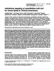
Figure 2.—Histogram of chromosomewise error probabilities (n ⫽ 54, interval size 0.1). __ indicates the expectation of the density under the assumption of all null hypotheses being true. – – – and ••• reflect the estimates of the proportion of the true null hypotheses estimated with FDRS and FDRB, respectively.

study that varied, from a practical point of view, only in the estimation of the proportion of true null hypotheses, ␲0. The FDRBH method assumes a ␲0-value of 1, which is in general not appropriate if the distribution of the P-values follows a mixture distribution, because in these cases there is information about the number of truly alternative hypotheses and thus also for ␲0. In the present study m is not very large compared to, for example, DNA microarray experiments. However, the distribution of the pc-values followed a mixture distribution as demonstrated in Figure 2. It can be observed that the proportion of pc-values with pc ⱕ 0.1 is significantly higher than would be expected if all null hypotheses were true. On the other hand, pc ⬎ 0.1 are almost uniformly distributed with a slight decrease with higher pcvalues. Additionally it is known from previous work that five QTL are real effects in the design that is the QTL for the five milk production traits on BTA14 (Thaller et al. 2003). Therefore, although m is not very large, a value of 1 for ␲0 as suggested by Benjamini and Hochberg (1995) is inappropriate and extremely conservative. Both the FDRS and the FDRB methods accounted for the mixture distribution of the pc-values, and both produced nearly identical results. Both methods estimated values for ␲0 (␲ ˆ 0,S ⫽ 0.30 and ␲ ˆ 0,B ⫽ 0.28) that are approximately in agreement with the density of the pcvalues for pc ⬎ 0.6 in the histogram in Figure 2. This density reflects the proportion of true null hypotheses (Storey and Tibshirani 2003). In his software manual Storey wrote that the FDRS method often works better than the FDRB method, but that it can backfire for a small number of tests or in pathological situations. In general, the authors recommended the use of the FDRB method if the number of tests is small. Similar to these two methods, Mosig et al. (2001) presented an iterative

algorithm for the estimation of the true null hypothesis that used the information of the mixture distribution of the pc-values and used this estimate for the calculation of the FDR. In this study, the method of Mosig et al. (2001) produced slightly higher q-values (not shown). The work of Storey and Tibshirani (2003) and Storey et al. (2004) in the field of the appropriate application of the FDR in genomics offered new possibilities to account for the problem of multiple testing in QTL mapping. The improved FDR provides a balance between the true and the false positive QTL by taking the mixture distribution of P-values into account. Furthermore, in the present study it also proved to be less conservative compared to the classical threshold setting. For example, when using the FDRB instead of the chromosomewise or even experimentwise threshold levels more QTL will be declared as significant (Table 4). Hence, replacing the classical threshold setting based on P-values by the presented FDR approach brings the number of declared QTL closer to the predicted number of Hayes and Goddard (2001). In summary, a large granddaughter design with progeny-tested sires from Germany and France was analyzed. The comparatively high number of QTL found emphasized the high power of the experiment. This high power was due to the large design, the inclusion of multiple QTL as cofactors in the statistical model, and the application of the false discovery rate, which accounted for the proportion of truly null hypotheses. As the analysis revealed no significant QTL-by-environment interaction the QTL found can be taken as candidates for the marker-assisted selection programs currently implemented in both countries, in Germany (Bennewitz et al. 2003b) as well as in France (Boichard et al. 2002). We thank Mike E. Goddard for helpful discussions and for carefully reading this manuscript. This article has benefited from the critical

Powerful QTL Analysis in Dairy Cattle comments of two anonymous reviewers. This research was supported by the German Cattle Breeders Federation and the German Ministry of Education, Science, Research and Technology.

LITERATURE CITED Benjamini, Y., and Y. Hochberg, 1995 Controlling the false discovery rate: a practical and powerful approach to multiple testing. J. R. Stat. Soc. Ser. B 85: 289–300. Benjamini, Y., and Y. Hochberg, 2000 On the adaptive control of false discovery rate in multiple testing with independent statistics. J. Educ. Behav. Stat. 25 (1): 60–83. Benjamini, Y., and D. Yekutieli, 1997 The control of the false discovery rate under dependence. Ann. Stat. 29 (4): 1165–1188. Bennewitz, J., N. Reinsch and E. Kalm, 2002 Improved confidence intervals in quantitative trait loci mapping by permutation bootstrapping. Genetics 160: 1673–1686. Bennewitz, J., N. Reinsch, C. Grohs, H. Leveziel, A. Malafosse et al., 2003a Combined analysis of data from two granddaughter designs: a simple strategy for QTL confirmation and increasing experimental power in dairy cattle. Genet. Sel. Evol. 35: 319–338. Bennewitz, J., N. Reinsch, H. Thomsen, J. Szyda, F. Reinhardt et al., 2003b Marker assisted selection in German Holstein dairy cattle breeding: outline of the program and marker assisted breeding value estimation. Session G1.9, 54th Annual Meeting of the European Association for Animal Production, August 31–September 3, Rome. Boichard, D., S. Fritz, M. N. Rossignol, M. Y. Boscher, A. Malafosse et al., 2002 Implementation of marker assisted selection in French dairy cattle breeding. Session 22–03, 7th World Congress on Genetics Applied to Livestock Production, August 19–23, Montpellier, France. Boichard, D., C. Grohs, F. Bourgeois, F. Cerqueira, R. Faugeras et al., 2003 Detection of genes influencing economic traits in three French dairy cattle breeds. Genet. Sel. Evol. 35: 1–25. Churchill, G. A., and R. W. Doerge, 1994 Empirical threshold values for quantitative trait mapping. Genetics 138: 963–971. De Koning, D. J., N. F. Schulman, K. Elo, S. Moisio, R. Kinos et al., 2001 Mapping of multiple quantitative trait loci by simple regression in half-sib designs J. Anim. Sci. 79: 616–622. Falconer, D. S., and T. F. C. Mackay, 1996 Introduction to Quantitative Genetics, Ed. 4. Longman Scientific & Technical, New York. Fernando, R. L., J. C. M. Dekkers and M. Soller, 2002 Controlling the proportion of false positive (PFP) in a multiple test genome scan for marker-QTL linkage. Session 21–37, 7th World Congress on Genetics Applied to Livestock Production, August 19–23, Montpellier, France. Go¨ring, H. H. H., J. D. Terwilliger and J. Blangero, 2001 Large upward bias in estimation of locus-specific effects from genomewide scans. Am. J. Hum. Genet. 69: 1357–1369. Green, P., K. Falls and S. Crooks, 1990 Documentation of CRI-MAP, Version 2.4. Washington University School of Medicine, St. Louis. Grisart, B., W. Coppieters, F. Farnir, L. Karim, C. Ford et al., 2002 Positional candidate cloning of a QTL in dairy cattle: identification of a missense mutation in the bovine DGAT1 gene with

1027

major effect on milk yield and composition. Genome Res. 12: 222–231. Hayes, B., and M. E. Goddard, 2001 The distribution of the effects of genes affecting quantitative traits in livestock. Genet. Sel. Evol. 33: 209–229. Hoeschele, I., P. Uimari, F. E. Grignola, Q. Zhang and K. M. Gage, 1997 Advances in statistical methods to map quantitative trait loci. Genetics 147: 1445–1457. Jansen, R. C., 1993 Interval mapping of multiple quantitative trait loci. Genetics 135: 205–211. Knott, S. A., J. M. Elsen and C. S. Haley, 1996 Methods for multiple-marker mapping of quantitative trait loci in half-sib populations. Theor. Appl. Genet. 93: 71–80. Lee, H., J. C. M. Dekkers, M. Soller, M. Malek, R. Fernando et al., 2002 Application of the false discovery rate to quantitative trait loci interval mapping with multiple traits. Genetics 161: 905–914. Mosig, M. O., E. Lipkin, G. Khutoreskaya, E. Tchourzyna, M. Soller et al., 2001 A whole genome scan for quantitative trait loci affecting milk protein percentage in Israeli-Holstein cattle, by means of selective milk DNA pooling in a daughter design, using an adjusted false discovery rate criterion. Genetics 157: 1683–1689. Reinsch, N., 1999 A multiple-species, multiple-project database for genotypes at co-dominant loci. J. Anim. Breed. Genet. 116: 425– 435. Storey, J. D., 2002 A direct approach to the false discovery rates. J. R. Stat. Soc. B 64: 479–498. Storey, J. D., and R. Tibshirani, 2003 Statistical significance for genome-wide studies. Proc. Natl. Acad. Sci. USA 100 (16): 9440– 9445. Storey, J. D., J. E. Taylor and D. Siegmund, 2004 Strong control, conservative point estimation, and simultaneous conservative consistency of false discovery rates: a unified approach. J. R. Stat. Soc. B 66 (1): 187–205. Thaller, G., W. Kra¨mer, A. Winter, B. Kaupe, G. Erhardt et al., 2003 Effects of DGAT1 variants on milk production traits in German cattle breeds. J. Anim. Sci. 81: 1911–1918. Thomsen, H., N. Reinsch, N. Xu, C. Looft, S. Grupe et al., 2000 A male bovine linkage map for the ADR granddaughter design. J. Anim. Breed. Genet. 117: 289–306. Thomsen, H., N. Reinsch, N. Xu, C. Looft, S. Grupe et al., 2001 Comparison of estimated breeding values, daughter yield deviations and de-regressed proofs within a whole genome scan for QTL. J. Anim. Breed. Genet. 118: 357–370. Weller, J. I., Y. Kashi and M. Soller, 1990 Power of daughter and granddaughter designs for determining linkage between marker loci and quantitative trait loci in dairy cattle. J. Dairy Sci. 73: 2525–2537. Weller, J. I., J. Z. Song, D. W. Heyen, H. A. Lewin and M. Ron, 1998 A new approach to the problem of multiple comparisons in the genetic dissection of complex traits. Genetics 150: 1699– 1706. Winter, A., W. Kramer, F. A. Werner, S. Kollers, S. Kata et al., 2002 Association of a lysine-232/alanine polymorphism in a bovine gene encoding acyl-CoA:diacylglycerol acyltransferase (DGAT1) with variation at a quantitative trait locus for milk fat content. Proc. Natl. Acad. Sci. USA 99 (14): 9300–9305. Communicating editor: C. Haley