Multiregion Image Segmentation by Parametric Kernel ... - CiteSeerX

IEEE TRANSACTIONS ON IMAGE PROCESSING, VOL. 20, NO. 2, FEBRUARY 2011

545

Multiregion Image Segmentation by Parametric Kernel Graph Cuts Mohamed Ben Salah, Member, IEEE, Amar Mitiche, Member, IEEE, and Ismail Ben Ayed, Member, IEEE

Abstract—The purpose of this study is to investigate multiregion graph cut image partitioning via kernel mapping of the image data. The image data is transformed implicitly by a kernel function so that the piecewise constant model of the graph cut formulation becomes applicable. The objective function contains an original data term to evaluate the deviation of the transformed data, within each segmentation region, from the piecewise constant model, and a smoothness, boundary preserving regularization term. The method affords an effective alternative to complex modeling of the original image data while taking advantage of the computational benefits of graph cuts. Using a common kernel function, energy minimization typically consists of iterating image partitioning by graph cut iterations and evaluations of region parameters via fixed point computation. A quantitative and comparative performance assessment is carried out over a large number of experiments using synthetic grey level data as well as natural images from the Berkeley database. The effectiveness of the method is also demonstrated through a set of experiments with real images of a variety of types such as medical, synthetic aperture radar, and motion maps. Index Terms—Graph cuts, image segmentation, kernel k-means.

I. INTRODUCTION

I

MAGE segmentation is a fundamental problem in computer vision. It has been the subject of a large number of theoretical and practical studies [1]–[3]. Its purpose is to divide an image into regions answering a given description. Many studies have focused on variational formulations because they result in the most effective algorithms [4]–[11]. Variational formulations [4] seek an image partition which minimizes an objective functional containing terms that embed descriptions of its regions and their boundaries. The literature abounds of both continuous and discrete formulations. Continuous formulations view images as continuous functions over a continuous domain [4]–[6]. The most effective minimizes active curve functionals via level sets [2], [3], [6]. The minimization relies on gradient descent. As a result, the algorithms converge to a local minimum, can be affected by the initialization [6], [12], and are notoriously slow in spite of the Manuscript received October 27, 2009; revised June 03, 2010; accepted August 05, 2010. Date of publication August 16, 2010; date of current version January 14, 2011. The associate editor coordinating the review of this manuscript and approving it for publication was Dr. Ferran Marques. M. Ben Salah and A. Mitiche are with the Institut National de la Recherche Scientifique (INRS-EMT), Montréal, H5A 1K6, QC, Canada (e-mail: [email protected]; [email protected]). I. Ben Ayed is with General Electric (GE) Canada, London, N6A 4V2, ON, Canada (e-mail: [email protected]). Color versions of one or more of the figures in this paper are available online at http://ieeexplore.ieee.org. Digital Object Identifier 10.1109/TIP.2010.2066982

various computational artifacts which can speed their execution [13]. The long time of execution is the major impediment in many applications, particularly those which deal with large images and segmentations into a large number of regions [12]. Discrete formulations view images as discrete functions over a positional array [9], [14]–[16], [18], [19]. Combinatorial optimization methods which use graph cut algorithms have been the most efficient. They have been of intense interest recently as several studies have demonstrated that graph cut optimization can be useful in image analysis. Very fast methods have been implemented for image segmentation [15], [20]–[25], motion and stereo segmentation [26], [27], tracking [28], and restoration [11], [14]. Following the work in [10], objective functionals typically contain a data term to measure the conformity of the image data within the segmentation regions to statistical models and a regularization term for smooth segmentation boundaries. Minimization by graph cuts of objective functionals with a piecewise constant data term produce nearly global optima [11] and, therefore, are less sensitive to initialization. Unsupervised graph cut methods, which do not require user intervention, have used the piecewise model, or its Gaussian generalization, because the data term can be written in the form required by the graph cut algorithm [11], [25], [29], [30]. However, although useful, these models are not generally applicable. For instance SAR images are best described by the Gamma distribution [31]–[33] and polarimetric images the Wishart distribution or the complex Gaussian [12], [34]. Even within the same image, different regions may require completely different models. For example, the luminance within shadow regions in sonar imagery is well modeled by the Gaussian distribution whereas the Rayleigh distribution is more accurate in the reverberation regions [35]. The parameters of all such models do not depend upon the data in a way that would preserve the form of the data term required by the graph cut algorithm and, as a result, the models cannot be used. The form of the objective function must be a sum over all pixels of pixel or pixel neighborhood dependent data and variables. Variables which are global over the segmentation regions do not apply if they cannot be written in a way that affords such a form. The parameters of a Gaussian are, in discrete approximation, linear combinations of image data and, as a result, can be used in the objective function. One way to introduce more general models is to allow user interaction. Several interactive graph cut methods have used models more general than the Gaussian by adding a process to learn the region parameters at any step of the graph cut segmentation process. These parameters become part of the data at

1057-7149/$26.00 © 2011 IEEE

546

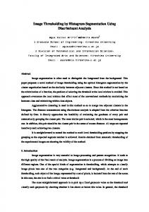
Fig. 1. Illustration of nonlinear 3-D data separation with mapping. Data is nonlinearly separable in the data space. The data is mapped to a higher dimensional feature (kernel) space so as to have a better separability, ideally linear. For the purpose of display, the feature space in this example is of the same dimension as the original data space. In general, the feature space is of higher dimension.

each step. However, the parameter learning and the segmentation process are only loosely coupled in the sense that they do not result from the objective function optimization. Current interactive methods have treated the case of the foreground/background segmentation, i.e., the segmentation into two regions. The studies in [10], [14] have described the regions by their image histograms and [17], [18] used mixtures of Gaussians. Although very effective in several applications, for instance image editing, interactive methods do not extend readily to multiregion segmentation into a large number of regions, where user interactions and general models, such as histograms and mixtures of Gaussians, become intractable. Note that it is always possible to use a given model in unsupervised graph cut segmentation if this model were learned beforehand. In this case, the model becomes part of the data. However, modeling is notoriously difficult and time consuming [36]. Moreover, a model learned using a sample from a class of images is generally not applicable to images of a different class. The purpose of this study is to investigate kernel mapping to bring the unsupervised graph cut formulation to bear on multiregion segmentation of images more general than Gaussian. The image data is mapped implicitly via a kernel function into data of a higher dimension so that the piecewise constant model, and the unsupervised graph cut formulation thereof, becomes applicable (see Fig. 1 for an illustration). The mapping is implicit because the dot product, the Euclidean norm thereof, in the higher dimensional space of the transformed data can be expressed via the kernel function without explicit evaluation of the transform [37]. Several studies have shown evidence that the prevalent kernels in pattern classification are capable of properly clustering data of complex structure [37]–[43]. In the view that image segmentation is spatially constrained clustering of image data [44], kernel mapping should be quite effective in segmentation of various types of images. The proposed functional contains two terms: an original kernel-induced term which evaluates the deviation of the mapped image data within each region from the piecewise constant model and a regularization term expressed as a function of the region indices. Using a common kernel function, the objective functional minimization is carried out by iterations of two

IEEE TRANSACTIONS ON IMAGE PROCESSING, VOL. 20, NO. 2, FEBRUARY 2011

consecutive steps: 1) minimization with respect to the image segmentation by graph cuts and 2) minimization with respect to the regions parameters via fixed point computation. The proposed method shares the advantages of both simple modeling and graph cut optimization. Using a common kernel function, we verified the effectiveness of the method by a quantitative and comparative performance evaluation over a large number of experiments on synthetic images. In comparisons to existing graph cut methods, the proposed method brings advantages in regard to segmentation accuracy and flexibility. To illustrate these advantages, we also ran the tests with various classes of real images, including natural images from the Berkeley database, medical images, and satellite data. More complex data, such as color images and motion maps, have also been used. The remainder of this paper is organized as follows. The next section reviews graph cut image segmentation commonly stated as a maximum a posteriori (MAP) estimation problem [10], [14], [17], [29]. Section III introduces the kernel-induced data term in the graph cut segmentation functional. It also gives functional optimization equations and the ensuing algorithm. Section IV describes the validation experiments, and Section V contains a conclusion. II. UNSUPERVISED PARAMETRIC GRAPH CUT SEGMENTATION be an image Let function from a positional array to a space of photometric variables such as intensity, disparities, color or texture vectors. regions consists of finding a partition Segmenting into of the discrete image domain so that each region is homogeneous with respect to some image characteristics. Graph cut methods state image segmentation as a label assignment problem. Partitioning of the image domain amounts to assigning each pixel a label in some finite set of labels . A region is defined as the set of pixels whose label is , i.e., is labeled . The problem consists of finding the labeling which minimizes a given functional describing some common constraints. Following the pioneer work of Boykov and Jolly [10], functionals which are often used and which arise in various computer vision problems are the sum of two characteristic terms: a data term to measure the conformity of image data within the segmentation regions to a statistical model and a regularization term (the prior) for smooth regions boundaries. Definition of the data term is crucial to the ensuing algorithms and is the main focus of this study. In this connection, several existing methods state image segmentation as a MAP estimation problem [10], [14], [17], [18], [25], [29], [30], [45]–[47], where optimization of the region term amounts to maximizing the conditional probability of pixel data given . In the assumed model distributions within regions, the context of interactive image segmentation, these model distributions are estimated from user interactions [14], [17], [18]. In this connection, Histograms [14] and mixture of Gaussian models (MGM) [17] are commonly used to estimate model distributions. In the context of unsupervised image segmentation, i.e., segmentation without user interactions, some parametric distributions, such as the Gaussian model, were amenable to

SALAH et al.: MULTIREGION IMAGE SEGMENTATION BY PARAMETRIC KERNEL GRAPH CUTS

graph cut optimization [29], [30]. To write down the segmentation functional, let be an indexing function. assigns each point of the image to a region

(1) where is the finite set of region indices whose cardinality is . The segmentation functional can then be less or equal to written as (2) where is the data term and the prior. is a positive factor. The MAP formulation using a given parametric model defines the data term as follows:

547

and, therefore, solve a (simpler) linear problem (refer to Fig. 1). More importantly, there is no need to explicitly compute the mapping . Using the Mercer’s theorem [37], the dot product in the feature space suffices to write the kernel-induced data term as a function of the image, the regions parameters, and a kernel function. Furthermore, neither prior knowledge nor user interactions are required for the proposed method. A. Proposed Functional Let be a nonlinear mapping from the observation space to a higher (possibly infinite) dimensional feature/mapped space . A given labeling assigns each pixel a label and, consequently, divides the image domain into multiple regions. Each region is characterized by one label: . Solving image segmentation in a kernel-induced space with graph cuts consists of finding the labeling which minimizes

(3) In this statement, the piecewise constant segmentation model, a particular case of the Gaussian distribution, has been the focus of several recent studies [11], [29], [30] because the ensuing algorithms are computationally simple. Let be the piecewise constant model parameter of region . In this case, the data term is given by (4) The prior is expressed as follows: (5) with a neighborhood set containing all pairs of neighboring is a smoothness regularization funcpixels and tion given by the truncated squared absolute difference [11], where [21], [29] is a constant. Although used most often, the piecewise constant model is, generally, not applicable. For instance, natural images require more general models [48], and the specific, yet important, SAR and polarimetric images require the Rayleigh and Wishart models [12], [31], [32]. In the next section, we will introduce a data term which references the image data transformed via a kernel function, and explain the purpose and advantages of doing so. III. SEGMENTATION FUNCTIONAL IN THE KERNEL INDUCED SPACE In general, image data is complex. Therefore, computationally efficient models, such as the piecewise Gaussian distribution, are not sufficient to partition nonlinearly separable data. This study uses kernel functions to transform image data: rather than seeking accurate (complex) image models and addressing a non linear problem, we transform the image data implicitly via a mapping function , typically nonlinear, so that the piecewise constant model becomes applicable in the mapped space

(6) measures kernel-induced non Euclidean distances between for the observations and the regions parameters . In machine learning, the kernel trick consists of using a linear classifier to solve a nonlinear problem by mapping the original nonlinear data into a higher dimensional space. Following the Mercer’s theorem [37], which states that any continuous, symmetric, positive semidefinite kernel function can be expressed as a dot product in a high-dimensional space, we do not have to know explicitly the mapping . Instead, we can use a kernel function, , verifying (7) where “ ” is the dot product in the feature space. Substitution of the kernel functions gives

(8) which is a nonEuclidean distance measure in the original data space corresponding to the squared norm in the feature space. Now, the simplifications in (8) lead to the following kernelinduced segmentation functional

(9) The functional (9) depends both upon regions parameters, , and the labeling . In the next subsection, we describe the segmentation functional optimization strategy.

548

IEEE TRANSACTIONS ON IMAGE PROCESSING, VOL. 20, NO. 2, FEBRUARY 2011

B. Optimization

TABLE I EXAMPLES OF PREVALENT KERNEL FUNCTIONS

Functional (9) is minimized with an iterative two-step optimization strategy. Using a common kernel function, the first step consists of fixing the labeling (or the image partition) and with respect to statistical regions parameters optimizing via fixed point computation. The second step consists of finding the optimal labeling/partition of the image, given region parameters provided by the first step, via graph cut iterations. The algorithm iterates these two steps until conwith respect to a parameter. vergence. Each step decreases Thus, the algorithm is guaranteed to converge at least to a local minimum. 1) Update of the Region Parameters: Given a partition of the with respect to , , image domain, the derivative of yields the following equations:

(10)

For each pixel , the -neighborhood system we adopt, , is of size 4, i.e., it is compound of the four horizontally and vertibe the set of neighbors of cally adjacent pixels to . Let verifying and . Then (10) can be written as

(11)

The sum in (11) can be restricted to pixels laying on the of each region . Indeed, for a pixel in the inboundary , i.e., and , all neighbors belong to terior of so that . This simplifies (11) to

Table I lists commonly used kernel functions [39]. In all our large number of experiments, we used the radial basis function (RBF) kernel. The RBF kernel has been prevalent in pattern data clustering [39], [43], [59]. With this kernel, the necessary condition for a minimum of the segmentation functional

with respect to region parameter fixed-point equation:

,

, is the following

(12) where

(13) and designates set cardinality. A proof of the existence of a fixed point is given in the Appendix A. Therefore, a minimum with respect to the region parameters can be computed by of gradient descent or fixed-point iterations using (12). The RBF kernel, although simple, yields outstanding results on a large set of experiments with images of various types (see the experimental Section IV). Also, note that, obviously, this RBF kernel method does not reduce to the gaussian model methods commonly used in the literature [17], [29]. The difference can be clearly seen in the fixed point update of the region parameters in (12) which, in the case of the Gaussian model, would be the simple mean update inside each region. 2) Update of the Partition With Graph Cut Optimization: In each iteration of this algorithm, the first step, described previously, is followed by a second step which minimizes the segmentation functional with respect to the partition of the image domain. The second step, based upon graph cut optimization, . In the following, seeks the labeling minimizing functional we give some basic definitions and notations. For easier referral to the graph cut literature, we will use the word label to mean region index. be a weighted graph, where is the set of Let vertices (nodes) and the set of edges. contains a node for each pixel in the image and two additional nodes called terminals. Commonly, one is called source and the other is called sink. between any two distinct nodes and . There is an edge is a set of edges verifying: A cut ; • terminals are separated in the graph . • no subset of separates terminals in This means that a cut is a set of edges the removal of which separates the terminals into two induced subgraphs. In addition, this cut is minimal in the sense that none of its subsets separates the terminals into the same two subgraphs. The minimum cut problem consists of finding the cut , in a given graph, , equals with the lowest cost. The cost of a cut, denoted the sum of its edge weights. By setting properly the weights of graph , one can use swap moves from combinatorial optimization [11] to compute efficiently minimum cost cuts corre. For each pair of sponding to a local minimum of functional , swap moves find the minimum cut in the subgraph labels

SALAH et al.: MULTIREGION IMAGE SEGMENTATION BY PARAMETRIC KERNEL GRAPH CUTS

549

TABLE II WEIGHTS ASSIGNED TO THE EDGES OF THE GRAPH FOR MINIMIZING THE PROPOSED FUNCTIONAL WITH RESPECT TO THE PARTITION

. The set is equal to , i.e., of vertices labeled or and termiit consists of the set consists of edges connecting nodes of nals and . The set between them and to terminals and . Given region parameters provided by the first step, this step consists of iterating the search for the minimum cut on the subover all pairs of labels. To do so, the graph weights graph need to be set dynamically whenever region parameters and the pair of labels change. Table II shows the weights assigned to the graph edges for minimizing functional (9) with respect to the partition.

Fig. 2. Image intensity distributions. (a) Small overlap. (b) Significant overlap.

IV. EXPERIMENTAL RESULTS Recall that the intended purpose of the proposed parametric kernel graph cut method (KM) is to afford an alternative image modeling by implicitly mapping the image data by a kernel function so that the piecewise constant model becomes applicable. Therefore, the purpose of this experimentation is to show how KM can segment images of a variety of types without an assumption regarding image model or models. To this end, we have two types of validation tests: 1) quantitative verification, via pixel misclassification frequency, using: • synthetic images of various models; • multimodel images, i.e., images composed of regions each of a different model; • simulations of real images such as SAR. 2) real images of three types: • SAR, which are best modeled by a Gamma distribution; • medical/polarimetric, which are best modeled by a Wishart distribution; • natural images of the Berkeley database—these results will be evaluated quantitatively using the provided multioperator manual segmentations. Additional experiments using vectorial images, namely color and motion, will also be given. A. Performance Evaluation With Synthetic Data In this subsection, we first show two typical examples of our large number of experiments with synthetic images and define the measures we adopted for performance analysis: the contrast and the percentage of misclassified pixels (PMP). Fig. 3(a) and (d) depicts two different versions of a two-region synthetic image, each perturbed with a Gamma noise. In the first version [Fig. 3(a)], noise parameters result in a small overlap (significant contrast) between the intensity distributions within the regions as shown in Fig. 2(a). In the second version [Fig. 3(d)], there is

Fig. 3. Segmentation of two Gamma noisy images with different contrasts. (a),(d) Noisy images with different contrasts. (b),(e) Segmentation boundary results with PGM. (c),(f) segmentation results with KM. Images size: 128 128.

2

a significant overlap between the intensity distributions as depicted in Fig. 2(b). The larger the overlap, the more difficult the segmentation [50]. The piecewise constant segmentation method and its piecewise Gaussian generalization have been the focus of most studies and applications [11], [29], [30], [51] because of their tractability. In the following, evaluation of the proposed method, referred to as kernelized method (KM), is systematically supported by comparisons with the piecewise Gaussian method (PGM). The PGM was used first to segment, as depicted in Fig. 3(b) and (e), the two versions of the two-region image with different contrast values. As the actual noise model is a Gamma model, segmentation quality obtained with the PGM was significantly affected when the contrast is small in Fig. 3(e). However, the KM yielded almost the same results quality for both images [Fig. 3(c) and3(f)], although the second image undergoes a significant overlap between the intensity distributions within the two regions as shown in Fig. 2(b). The previous example, although simple, showed that, without assumptions as to the images model, the KM can segment images whose noise model is different from piecewise Gaussian. To demonstrate that the KM is a flexible and effective alternative to image modeling, we proceeded to a quantitative and comparative performance evaluation over a very large number

550

IEEE TRANSACTIONS ON IMAGE PROCESSING, VOL. 20, NO. 2, FEBRUARY 2011

Fig. 4. (a) Synthetic images with Gamma (first row) and Exponential (second row) noises. (b) Segmentation boundary results with PGM. (c) Segmentation adapted to the actual noise model; and (d) The KM. Image size: 241 183.

2

of experiments. We generated more than 100 versions of a synthetic two-region image, each of them is the combination of a noise model and a contrast value. The noise models we used include the Gaussian, exponential and Gamma distributions. We segmented each image with the PGM, the KM and the actual noise model, i.e., the noise model used to generate the image at hand.1 The contrast values were measured by the Bhattacharyya distance between the intensity distributions within the two regions of the actual image [50] (14) where and denote the intensity distributions within the is the Bhattacharyya cotwo regions and efficient measuring the amount of overlap between these distributions. Small values of the contrast measure , correspond to images with high overlap between the intensity distributions within the regions. We carried out a comparative study by assessing the effect of the contrast on segmentation accuracy for the three segmentations methods. We evaluated the accuracy of segmentations via the percentage of misclassified pixels (PMP) defined, in the two-region segmentation case, as (15) where and denote the background and foreground of the ground truth (correct segmentation) and and denote the background and foreground of the segmented image. One example from the set of experiments we ran on synthetic data is depicted in Fig. 4. We show two different noisy versions of a piecewise constant two-region image perturbed with a Gamma (first row) and exponential noises (second row). The overlap between the intensity distributions within regions is relatively important in both images of Fig. 4(a). Indeed, the , and the expoGamma noisy image has a contrast of . The nentially noisy image (second row) a contrast of 1By the method using the actual noise model, we mean the method adapted for the noise model of the image at hand. For example, if we treat a synthetic image perturbed with a Gamma noise, the PGM and KM are compared together with the segmentation method where the parametric conditional probability in (3) is supposed Gamma.

PGM yielded unsatisfactory results [Fig. 4(b)]; the percentage of misclassified pixels was 36% for the Gamma noise and 42% for the exponential noise. The white contours are not visible because the regions they enclose are very small. When the correct model is assumed2 [Fig. 4(c)], better results were obtained. Although no assumption was made as to the noise model, the KM yielded a competitive segmentation quality [Fig. 4(d)]. For instance, in the case of the image perturbed with an exponential noise, the method adapted to the actual model, i.e., the exponential distribution, yielded a PMP equal to 5.2% wheras the KM yielded a PMP less than 2.6% for both noisy images. The proposed method allows much more flexibility in practice because the model distribution of image data and its parameters do not have to be fixed. Our comparative study investigated the effect of the contrast on the PMP over more than 100 experiments. Several synthetic two-region images were generated from the Gaussian, Gamma and exponential noises. For each noise model, the contrast between the two regions was varied gradually, which yielded more than 30 versions. For each image, we evaluated the segmentation accuracy, via the PMP, for the three segmentation methods: The KM, the PGM, and segmentation when the correct model and its parameters are assumed, i.e., the model and parameters used to generate the image of interest. First, we segmented the subset of images perturbed with the Gaussian noise using both the KM and PGM methods, and displayed the PMP as a function of the contrast [Fig. 5(a)]. In this case, the actual model is the piecewise Gaussian model which corresponds to the PGM. Therefore; we plotted only two curves. The higher the PMP, the higher the segmentation error and the poorer the segmentation quality. Although fully unsupervised, the KM yielded approximately the same error as segmentation with the correct model whose parameters are learned in advance, i.e., the Gaussian model in this case. 2Note that, for comparisons, embedding models such Gamma and exponential in the data term is not directly amenable to graph cut optimization. Instead, we assume that these parametric distributions are known beforehand. This is similar to several previous studies which used interactions to estimates the distributions of the segmentation regions. The negative log-likelihood of these distributions is, thus, used to set regional penalties in the data term [10], [14], [23]. Note that assuming that regions distributions are known beforehand is in favor of the methods we compared with and, therefore, would not bias the comparative appraisal of the proposed kernel method.

SALAH et al.: MULTIREGION IMAGE SEGMENTATION BY PARAMETRIC KERNEL GRAPH CUTS

551

Fig. 5. Evaluation of segmentation error for different methods over a large number of experiments (PMP as a function of the contrast): comparisons over the subset of synthetic images perturbed with a Gaussian noise in (a), the exponential noise in (b), and the Gamma noise in (c).

Fig. 7. (a) Simulated multilook SAR image. (b) Segmentation at convergence with KM. (c)–(f) Segmentation regions separately.  : . Image size: 512 512.

2

Fig. 6. Image with different noise models. (a) Noisy image. (b) Segmentation boundary at convergence. (c) Regions labels at convergence. (d)–(f) Segmentation regions separately. (h) Segmentation boundary at convergence with the for both methods. PGM. (i) Regions labels at convergence with PGM.  Image size: 163 157. Note that a value of parameter  approximately equal to 2 is shown to be optimal for distributions from the exponential family such as the piecewise Gaussian model [50]. The study in [50] shows that this value corresponds to the minimum of the mean number of misclassified pixels, and has an interesting minimum description length (MDL) interpretation.

2

=2

Second, we segmented the set of images perturbed with the exponential noise with PGM, KM and the method adapted to the actual model, i.e., the exponential model in this case. In Fig. 5(b), the PMP is plotted as a function of the contrast. The PGM undergoes a high error gradient at some Bhattacharyya distance. This is consistent with the level set segmentation experiments in [49], [50]. When is superior to 0.55, all methods yield a low segmentation error with a PMP less than 5%. When , the KM outperforms clearly the contrast decreases the PGM and behaves like the correct model for a large range of Bhattacharyya distance values [refer to Fig. 5(b)]. Similar experiments were run with the set of images perturbed with a Gamma noise, and a similar behavior was observed [refer to Fig. 5(c)]. These results demonstrate that the KM can deal with various classes of image noises and very small contrast values. It yields competitive results in comparison to using the correct model, neither the model nor its parameters

= 05

were learned a priori. This is an important advantage of the proposed method-it relaxes assumptions as to the noise model and, therefore, is a flexible alternative to image modeling. Another important advantage of the KM is the ability to segment multimodel images, i.e., images whose regions require different models. For instance, this can be the case with synthetic aperture radar (SAR) images where the intensity follows a Gamma distribution in a zone of constant reflectivity and a K distribution in a zone of textured reflectivity [52]. The luminance within shadow regions in sonar imagery is well modeled by the Gaussian distribution while the Rayleigh distribution is more accurate in the reverberation regions [35]. To demonstrate the ability of KM to process multimodel images, consider the synthetic image of three regions, each with a different noise model in Fig. 6(a). A Gaussian distributed noise has been added to the clearer region, a Rayleigh distributed noise to the gray, and a Poisson distributed noise to the darker region. The final segmentation (i.e., at convergence) with the KM is displayed in Fig. 6(b) where each region is delineated by a colored curve. Fig. 6(c) shows each region, in the final segmentation, represented by its corresponding label and Fig. 6(d)–6(f) show the segmentation regions separately. As expected, the PGM yielded corrupted segmentation results [see the segmentation regions at convergence in Fig. 6(h), and/or the labels at convergence in Fig. 6(i)]. This experiment demonstrates that the KM can discriminate different distributions within one single image.

552

IEEE TRANSACTIONS ON IMAGE PROCESSING, VOL. 20, NO. 2, FEBRUARY 2011

Fig. 8. (a) Monolook SAR image. (b) Segmentation boundary at convergence with KM. (c) Segmentation labels. (d) Segmentation boundary at convergence with PGM. Values of  were set for each method in order to give the best results. Image size: 361 151.

2

Fig. 9. (a) SAR image of the Flevoland region. (b) Segmentation boundary at convergence. (c) Segmentation labels. 

The preceding example used a multimodel image with additive noise. The purpose of this next example is to show that KM is also applicable to multimodel images with multiplicative noise such as SAR. It is generally recognized that the presence of multiplicative speckle noise is the single most complicating factor in SAR segmentation [31]–[33]. Fig. 7(a) depicts an amplitude 8-look3 synthetic 512 512 SAR image compound of four regions. The KM was applied with an initialization of four regions with their parameters chosen arbitrarily. The purpose of this experiment, is to show the ability of the KM to adapt systematically to this kind of noise model. Fig. 7(b) depicts final segmentation regions, each represented by its label at convergence. These segmentation regions are displayed separately in Fig. 7(c)–7(f). B. Real Data The following experiments demonstrate KM applied to three different types of images: SAR, polarimetric/medical, and the images of the Berkeley database. We also include additional experiments with vectorial images, namely color and motion.

= +

3In single-look SAR images, the intensity is given by I a b , where a and b denote the real and imaginary parts of the complex signal acquired from the radar. For multilook SAR images, the L-look intensity is the average of the L intensity images [31].

= 0:8. Image size: 512 2 800.

1) SAR and Polarimetric/Medical Images: As mentioned earlier, SAR image segmentation is generally acknowledged to be difficult [31], [48] because of the multiplicative speckle noise. We also recall that SAR images are best modeled by Gamma distribution [31]. Fig. 8(a) depicts a monolook SAR image where the contrast is very low in many spots of the image. Detecting the edges of the object of interest, in such case, is very sensible. In Fig. 8(b), we show the final segmentation of this image into two regions, where the region of interest is delineated by the colored curve. In Fig. 8(c), each region is (corresponding to label ) at represented by its parameter convergence. As we can see, the PGM produces unsatisfactory results although we used the value of parameter which gives the best visual result. Another example of real SAR images is given in Fig. 9(a). This SAR image depicts the region of Flevoland in Netherland. Fig. 9(b)–(c) depicts, respectively, the final segmentation and segmentation regions represented with their parameters at convergence. This next example uses medical/polarimetric images, best modeled by a Wishart distribution [12]. The brain image, shown in Fig. 10(a), was segmented into three regions. In this case, the choice of the number of regions is based upon prior medical knowledge. Segmentation at convergence and final labels are displayed as in previous examples. Fig. 10(d) depicts a spot of very narrow human vessels with very small contrast within

SALAH et al.: MULTIREGION IMAGE SEGMENTATION BY PARAMETRIC KERNEL GRAPH CUTS

553

TABLE III AVERAGE PERFORMANCES OF THE KM METHOD AGAINST FIVE UNSUPERVISED ALGORITHMS IN TERMS OF THE PRI AND VOI MEASURES ON THE BERKELEY DATABASE [58]. THE FIRST LINE CORRESPONDS TO PERFORMANCES OF HUMAN OBSERVERS

Fig. 10. Brain and Vessel images. (a),(d) Original images. (b),(e) Segmentations at convergence. (c),(f) Final labels.

some regions. The results obtained in both cases are satisfying. The most important aim of this experiment is to demonstrate the ability of the proposed method to adapt automatically to this class of images acquired with special techniques other than the common ones. These results with gray level images show that the proposed method is robust and flexible; it can deal with various types of images. 2) Natural Images-Berkeley Database: We compare the KM against five unsupervised algorithms which are publicly available on natural images from the Berkeley database: Mean-Shift [53], NCuts [9], CTM [54], FH [55], and PRIF [56]. As our purpose is to address a variety of image models, we perform also comparative tests on the synthetic dataset used in Section IV-A to study the ability of these methods to adapt to different noise models. These comparisons are based basically on two performance measures which seem to be among the most correlated with human segmentation in term of visual perception: The probabilistic rand index (PRI) and the variation of information (VoI)4 [54], [57]. Since all methods are unsupervised, we use both training and test images in the Berkeley database which consists of 300 color images of size 481 321. To measure the accuracy of the results, a set of benchmark segmentation results provided by four to seven human observers for each image are available [58]. The PRI is conceived to take into account this variability of segmentations between human observers as it, not only, counts the number of pairs of pixels whose labels are consistent between automatic and ground truth segmentations, but also averages with regard to various human segmentations [57]. For the comparative appraisal, internal parameters of the five used algorithms are set (as in [54]) to optimal values or to values suggested by the authors. These parameters are: for Mean-shift [53]; for NCuts for FH [55]; which gives [9]; the best PRI for CTM [54], and 4We used the Matlab codes provided by Allen Y. Yang to compute PRI and VoI measures. This code is available on-line at http://www.eecs.berkeley.edu/ ~yang/software/lossy_segmentation/.

for PRIF [56]. As in [54], [56], the color images are normalized to have the longest side equal to 320 pixels due to memory issues. As the purpose of our method is to address various image noise models, we compare the KM on two datasets: the Berkeley database for natural images and the synthetic dataset containing images with three noise models: Gaussian, Gamma and exponential. In the first comparative study, we tested the KM against five unsupervised algorithms which are available on-line. After that, the two methods which obtained the best PRI scores in the first comparative study, PRIF and FH for instance, are tested against the KM on the synthetic database. The KM has been and run with an initial maximum number of regions . Note that, in this work, a rethe regularization weight gion is a set of pixels having the same label which is different from works in [54], [56], and [58] where it is rather a set of non connected pixels belonging to the same class. Experimentally, a agrees with the average number of segments value of from the human subjects. Table III shows the quantitative comparison of KM against the five other algorithms on the Berkeley benchmark. Values of , higher is better and VoI ranges in , lower PRI are in is better. The KM outperforms CTM, mean-shift, and NCuts in terms of the PRI indice although it is not conceived to specially work on natural images as the CTM does for example. The FH yields better performance than KM in terms of PRI but not the VoI. In terms of VoI, the KM outperforms mean-shift, NCuts, and FH. It is not surprising that the CTM yielded better VoI than the KM as it optimizes an information-theoretic criterion (recall that VoI measures the average conditional entropy of one segmentation given the other). PRIF is the unique method which yields the best results in terms of both measures. Based upon these performances in terms of the PRI, we also compared the KM with both PRIF and FH on images of the synthetic multimodel image dataset, images which are very different from natural images. We recall that these images are perturbed with Gaussian, Gamma, and exponential noises and the contrasts between the foreground and the background varies considerably (see Section IV-A). As shown in Table IV, the KM outperforms PRIF and FH algorithms in terms of both indices. We kept the same internal parameters used in the first comparison on Berkeley database for the three algorithms. This is mainly because the purpose is to compare the behavior of the

554

IEEE TRANSACTIONS ON IMAGE PROCESSING, VOL. 20, NO. 2, FEBRUARY 2011

Fig. 11. Examples of segmentations obtained by the KM algorithm on color images from Berkeley database. Although displayed in gray level, all the images are processed as color images.

TABLE IV AVERAGE PERFORMANCES OF THE KM METHOD AGAINST TWO UNSUPERVISED ALGORITHMS IN TERMS OF THE PRI AND VOI MEASURES ON THE SYNTHETIC DATASET OF SECTION IV-A

different methods regarding different kind of images without any specific tuning for each dataset. Overall, the KM reached competitive results as it gives relatively good results in terms of two segmentation indices for natural images, and the best results for the synthetic images compared to two state of the art algorithms. Fig. 12 depicts the distribution of the PRI indice corresponding to the KM over the

Fig. 12. Distribution of PRI measure of the KM applied to the images of , . Images size 320 214. Berkeley database.

N = 10  = 2

2

SALAH et al.: MULTIREGION IMAGE SEGMENTATION BY PARAMETRIC KERNEL GRAPH CUTS

555

Fig. 13. Segmentation of the Road and Marmor sequences. (a) Motion map of the Road sequence. (b) Segmentation at convergence of Road sequence. (c) Moving object segmentation region. (d) Motion map of Marmor sequence. (e) Segmentation at convergence of Marmor sequence. (f)-(g) Moving objects separately.

300 images of Berkeley database. Note the relative low variance especially for low scores standard deviation . For visual inspection, we show some examples of these segmentations obtained by the KM in Fig. 11. 3) Vectorial Data: In this part, we run experiments on vectorial images in order to test the effectiveness of the method for more complex data. We show a representative sample of the tests with motion sequences. Color images have been already treated in Section IV-B-II with the Berkeley database. In an -vectorial image, each pixel value is viewed as a vector of size . The kernels in Table I support vectorial data and, hence, may be applied directly. Motion sequences are the kind of vectorial data that we consider here for experimentation. In the following, we segment optical flow images into motion regions. Optical flow computed using the at each region is a 2-D vector method in [60]. We consider two typical examples: the Road image sequence (refer to the first row of Fig. 13) and the Marmor sequence (refer to the second row of Fig. 13). The Road sequence is compound of two regions: a moving vehicle and a background. Marmor sequence contains three regions: two moving objects in different directions and a background. The optical flow field is represented, at each pixel, by a vector as shown in Fig. 13(a) and (d). Final segmentations are shown in Fig. 13(b) and (e) where each moving object is delineated by a different colored curve. In Fig. 13(c), (f), and (g), we display the segmented moving objects separately.

synthetic images illustrated the flexibility and effectiveness of the proposed method. We have shown that the proposed approach yields competitive results in comparison with using the correct model learned in advance. Moreover, the flexibility and effectiveness of the method were tested over various types of real images including synthetic SAR images, medical and natural images, as well as motion maps. APPENDIX Consider the scalar function

(A.1)

where is the RBF kernel used in our experiments. In the following, we prove that this function has at least one fixed point. The continuous variable is a continuous grey level which, . Similarly, and typically, belongs to a given interval lay in the same interval. Hence, the following inequalities are automatically derived:

V. CONCLUSION This study investigated multiregion graph cut image segmentation in a kernel-induced space. The method consists of minimizing a functional containing an original data term which references the image data transformed via a kernel function. The optimization algorithm iterated two consecutive steps: graph cut optimization and fixed point iterations for updating the regions parameters. A quantitative and comparative performance study over a very large number of experiments on

(A.2) It results from these inequalities that is as follows: quently, the function

. Conse-

556

IEEE TRANSACTIONS ON IMAGE PROCESSING, VOL. 20, NO. 2, FEBRUARY 2011

Let us define the function

as follows:

One can easily note that . As is continuous (sum of continuous functions) over , there is at least one such that . Hence, the function has at as a fixed-point. least ACKNOWLEDGMENT The author would like to thank the two anonymous reviewers whose detailed comments and suggestions have contributed to improving both the content and the presentation quality of this paper. REFERENCES [1] J. M. Morel and S. Solimini, Variational Methods in Image Segmentation. Cambridge, MA: Birkhauser, 1995. [2] G. Aubert and P. Kornprobst, Mathematical Problems in Image Processing: Partial Differential Equations and the Calculus of Variations. New York: Springer-Verlag, 2006. [3] D. Cremers, M. Rousson, and R. Deriche, “A review of statistical approches to level set segmentation: Integrating color, texture, motion and shape,” Int. J. Comput. Vis., vol. 72, no. 2, pp. 195–215, 2007. [4] D. Mumford and J. Shah, “Optimal approximation by piecewise smooth functions and associated variational problems,” Comm. Pure Appl. Math, vol. 42, pp. 577–685, 1989. [5] S. C. Zhu and A. Yuille, “Region competetion: Unifying snakes, region growing, and bayes/MDL for multiband image segmentation,” IEEE Trans. Pattern Anal. Mach. Intell., vol. 18, no. 6, pp. 884–900, Jun. 1996. [6] T. F. Chan and L. A. Vese, “Active contours without edges,” IEEE Trans. Image Process., vol. 10, no. 2, pp. 266–277, Feb. 2001. [7] L. A. Vese and T. F. Chan, “A multiphase level set framework for image segmentation using the Mumford ans Shah model,” Int. J. Comput. Vis., vol. 50, no. 3, pp. 271–293, 2002. [8] V. Caselles, R. Kimmel, and G. Sapiro, “Geodesic active contours,” in Proc. Int. Conf. Comput. Vis., 1995, pp. 694–699. [9] J. Shi and J. Malik, “Normalized cuts and image segmentation,” IEEE Trans. Pattern Anal. Mach. Intell., vol. 22, no. 8, pp. 888–905, Aug. 2000. [10] Y. Boykov and M.-P. Jolly, “Interactive graph cuts for optimal boundary and region segmentation of objects in N-D images,” in Proc. IEEE Int. Conf. Comput. Vis., 2001, pp. 105–112. [11] Y. Boykov, O. Veksler, and R. Zabih, “Fast approximate energy minimization via graph cuts,” IEEE Trans. Pattern Anal. Mach. Intell., vol. 23, no. 11, pp. 1222–1239, Nov. 2001. [12] I. B. Ayed, A. Mitiche, and Z. Belhadj, “Polarimetric image segmentation via maximum-likelihood approximation and efficient multiphase level-sets,” IEEE Trans. Pattern Anal. Mach. Intell., vol. 28, no. 9, pp. 1493–1500, Sep. 2006. [13] J. A. Sethian, Level Set Methods and Fast Marching Methods, 2nd ed. Cambridge, U.K.: Cambridge Univ. Press, 1999. [14] Y. Boykov and G. Funka-Lea, “Graph cuts and efficient N-D image segmentation,” Int. J. Comput. Vis., vol. 70, no. 2, pp. 109–131, 2006. [15] Y. Boykov, V. Kolmogorov, D. Cremers, and A. Delong, “An integral solution to surface evolution PDEs via geo-cuts,” Proc. Eur. Conf. Comput. Vis., vol. 3, pp. 409–422. [16] Y. G. Leclerc, “Constructing simple stable descriptions for image partitioning,” Int. J. Comput. Vis., vol. 3, no. 1, pp. 73–102, 1989. [17] A. Blake, C. Rother, M. Brown, P. Perez, and P. Torr, “Interactive image segmentation using an adaptive GMMRF model,” in Proc. Eur. Conf. Comput. Vis., 2004, pp. 428–441. [18] C. Rother, V. Kolmogorovy, and A. Blake, “Grabcut-interactive foreground extraction using iterated graph cuts,” ACM Trans. Graph., pp. 309–314, 2004. [19] F. Destrempes, M. Mignotte, and J.-F. Angers, “A stochastic method for Bayesian estimation of hidden Markov random field models with application to a color model,” IEEE Trans. Image Process., vol. 14, no. 8, pp. 1096–1124, Aug. 2005.

[20] Y. Boykov and V. Kolmogorov, “An experimental comparison of min-cut/max-flow algorithms for energy minimization in vision,” IEEE Trans. Pattern Anal. Mach. Intell., vol. 26, no. 9, pp. 1124–1137, Sep. 2004. [21] O. Veksler, “Efficient graph-based energy minimization methods in computer vision,” Ph.D. dissertation, Cornell Univ., Ithaca, NY, 1999. [22] D. Freedman and T. Zhang, “Interactive graph cut based segmentation with shape priors,” in Proc. IEEE Int. Conf. Comput. Vis. Pattern Recognit., 2005, pp. 755–762. [23] S. Vicente, V. Kolmogorov, and C. Rother, “Graph cut based image segmentation with connectivity priors,” in Proc. IEEE Int. Conf. Comput. Vis. Pattern Recognit., Alaska, Jun. 2008, pp. 1–8. [24] P. Felzenszwalb and D. Huttenlocher, “Efficient graph-based image segmentation,” Int. J. Comput. Vis., vol. 59, pp. 167–181, 2004. [25] N. Vu and B. S. Manjunath, “Shape prior segmentation of multiple objects with graph cuts,” in Proc. IEEE Int. Conf. Comput. Vis. Pattern Recognit., 2008, pp. 1–8. [26] T. Schoenemann and D. Cremers, “Near real-time motion segmentation using graph cuts,” in Proc. DAGM Symp., 2006, pp. 455–464. [27] S. Roy, “Stereo without epipolar lines: A maximum-flow formulation,” Int. J. Comput. Vis., vol. 34, no. 2-3, pp. 147–162, 1999. [28] J. Xiao and M. Shah, “Motion layer extraction in the presence of occlusion using graph cuts,” IEEE Trans. Pattern Anal. Mach. Intell., vol. 27, no. 10, pp. 1644–1659, Oct. 2005. [29] M. B. Salah, A. Mitiche, and I. B. Ayed, “A continuous labeling for multiphase graph cut image partitioning,” in Advances in Visual Computing, Lecture Notes in Computer Science (LNCS), G. B. e. al, Ed. New York: Springer-Verlag, 2008, vol. 5358, pp. 268–277. [30] N. Y. El-Zehiry and A. Elmaghraby, “A graph cut based active contour for multiphase image segmentation,” in Proc. IEEE Int. Conf. Image Process., 2008, pp. 3188–3191. [31] I. B. Ayed, A. Mitiche, and Z. Belhadj, “Multiregion level-set partitioning of synthetic aperture radar images,” IEEE Trans. Pattern Anal. Mach. Intell., vol. 27, no. 5, pp. 793–800, May 2005. [32] E. E. Kuruoglu and J. Zerubia, “Modeling SAR images with a generalization of the Rayleigh distribution,” IEEE Trans. Image Processing, vol. 13, no. 4, pp. 527–533, Apr. 2004. [33] A. Achim, E. E. Kuruoglu, and J. Zerubia, “SAR image filtering based on the heavy-tailed Rayleigh model,” IEEE Trans. Image Process., vol. 15, no. 9, pp. 2686–2693, Sep. 2006. [34] A. A. Nielsen, K. Conradsen, and H. Skriver, “Polarimetric synthetic aperture radar data and the complex Wishart distribution,” in Proc. 13th Scandinavian Conf. Image Anal., Jun. 2003, pp. 1082–1089. [35] M. Mignotte, C. Collet, P. Pérez, and P. Bouthemy, “Sonar image segmentation using an unsupervised hierarchical MRF model,” IEEE Trans. Image Process., vol. 9, no. 7, pp. 1216–1231, Jul. 2000. [36] S. C. Zhu, “Statistical modeling and conceptualization of visual patterns,” IEEE Trans. Pattern Anal. Mach. Intell., vol. 25, no. 6, pp. 691–712, Jun. 2003. [37] K. R. Muller, S. Mika, G. Ratsch, K. Tsuda, and B. Scholkopf, “An introduction to kernel-based learning algorithms,” IEEE Trans. Neural Netw., vol. 12, no. 2, pp. 181–202, Mar. 2001. [38] A. Jain, P. Duin, and J. Mao, “Statistical pattern recognition: A review,” IEEE Trans. Pattern Anal. Mach. Intell., vol. 22, no. 1, pp. 4–37, Jan. 2000. [39] I. S. Dhillon, Y. Guan, and B. Kulis, “Weighted graph cuts without eigenvectors: A multilevel approach,” IEEE Trans. Pattern Anal. Mach. Intell., vol. 29, no. 11, pp. 1944–1957, Nov. 2007. [40] B. Scholkopf, A. J. Smola, and K. R. Muller, “Nonlinear component analysis as a kernel eigenvalue problem,” Neural Comput., vol. 10, pp. 1299–1319, 1998. [41] T. M. Cover, “Geomeasureal and statistical properties of systems of linear inequalities in pattern recognition,” Electron. Comput., vol. EC-14, pp. 326–334, Mar. 1965. [42] M. Girolami, “Mercer kernel based clustering in feature space,” IEEE Trans. Neural Netw., vol. 13, no. 3, pp. 780–784, May 2001. [43] D. Q. Zhang and S. C. Chen, “Fuzzy clustering using kernel methods,” in Proc. Int. Conf. Control Autom., Jun. 2002, pp. 123–127. [44] C. Vazquez, A. Mitiche, and I. B. Ayed, “Image segmentation as regularized clustering: A fully global curve evolution method,” in Proc. IEEE Int. Conf. Image Processing, Oct. 2004, pp. 3467–3470. [45] P. Kohli, J. Rihan, M. Bray, and P. H. S. Torr, “Simultaneous segmentation and pose estimation of humans using dynamic graph cuts,” Int. J. Comput. Vis., vol. 79, no. 3, pp. 285–298, 2008. [46] V. Kolmogorov, A. Criminisi, A. Blake, G. Cross, and C. Rother, “Probabilistic fusion of stereo with color and contrast for bilayer segmentation,” IEEE Trans. Pattern Anal. Mach. Intell., vol. 28, no. 9, pp. 1480–1492, Sep. 2006.

SALAH et al.: MULTIREGION IMAGE SEGMENTATION BY PARAMETRIC KERNEL GRAPH CUTS

[47] X. Liu, O. Veksler, and J. Samarabandu, “Graph cut with ordering constraints on labels and its applications,” in Proc. IEEE Int. Conf. Comput. Vis. Pattern Recognit., 2008, pp. 1–8. [48] I. B. Ayed, N. Hennane, and A. Mitiche, “Unsupervised variational image segmentation/classification using a weibull observation model,” IEEE Trans. Image Process., vol. 15, no. 11, pp. 3431–3439, Nov. 2006. [49] G. Delyon, F. Galland, and P. Refregier, “Minimal stochastic complexity image partitioning with unknown noise model,” IEEE Trans. Image Process., vol. 15, no. 10, pp. 3207–3212, Oct. 2006. [50] P. Martin, P. Refregier, F. Goudail, and F. Guerault, “Influence of the noise model on level set active contour segmentation,” IEEE Trans. Pattern Anal. Mach. Intell., vol. 26, no. 6, pp. 799–803, Jun. 2004. [51] X.-C. Tai, O. Christiansen, P. Lin, and I. Skjælaaen, “Image segmentation using some piecewise constant level set methods with MBO type of projection,” Int. J. Comput. Vis., vol. 73, no. 1, pp. 61–76, 2007. [52] R. Fjortoft, Y. Delignon, W. Pieczynski, M. Sigelle, and F. Tupin, “Unsupervised classification of radar images using hidden Markov chains and hidden Markov random fields,” IEEE Trans. Geosci. Remote Sens., vol. 41, no. 3, pp. 675–686, Mar. 2003. [53] D. Comaniciu and P. Meer, “Mean shift: A robust approach toward feature space analysis,” IEEE Trans. Pattern Anal. Mach. Intell., vol. 24, no. 5, pp. 603–619, May 2002. [54] Yang, Y. Allen, J. Wright, Y. Ma, and S. S. Sastry, “Unsupervised segmentation of natural images via lossy data compression,” Comput. Vis. Image Understand., vol. 110, no. 2, pp. 212–225, 2008. [55] P. Felzenszwalb and D. Huttenlocher, “Efficient graph-based image segmentation,” Int. J. Comput. Vis., vol. 59, no. 2, pp. 167–181, 2004. [56] M. Mignotte, “A label field fusion Bayesian model and its penalized maximum Rand estimator for image segmentation,” IEEE Trans. Image Process., vol. 19, no. 6, pp. 1610–1624, Jun. 2010. [57] R. Unnikrishnan, C. Pantofaru, and M. Hebert, “A measure for objective evaluation of image segmentation algorithms,” in Proc. IEEE Int. Conf. Comput. Vis. Pattern Recognit., Jun. 2005, vol. 3, pp. 34–41. [58] D. Martin and C. Fowlkes, The Berkeley Segmentation Database and Benchmark, Image Database and Source Code Publicly [Online]. Available: http://www.eecs.berkeley.edu/Research/Projects/CS/vision/grouping/segbench/ [59] P. J. Huber, Robust Statistics. New York: , 1981. [60] C. Vazquez, A. Mitiche, and R. Laganiere, “Joint multiregion segmentation and parametric estimation of image motion by basis function representation and level set evolution,” IEEE Trans. Pattern Anal. Mach. Intell., vol. 28, no. 5, pp. 782–793, May 2006.

557

Mohamed Ben Salah (S’09–M’10) was born in 1980. He received the State engineering degree from the École Polytechnique, Tunis, Tunisia, in 2003, the M.S. degree in computer science from the National Institute of Scientific Research (INRS-EMT), Montreal, QC, Canada, in 2006, and is currently pursuing the Ph.D. degree in computer science at INRS-EMT. His research interests are in image and motion segmentation with focus on level set and graph cut methods, and shape priors.

Amar Mitiche (M’09) received the Licence Ès Sciences in mathematics from the University of Algiers, Algiers, Algeria, and the Ph.D. degree in computer science from the University of Texas, Austin. He is currently a professor at the Institut National de Recherche Scientifique (INRS), Department of Telecommunications (INRS-EMT), Montreal, QC, Canada. His research is in computer vision. His current interests include image segmentation, motion analysis in monocular and stereoscopic image sequences (detection, estimation, segmentation, tracking, 3-D interpretation) with a focus on level set and graph cut methods, and written text recognition with a focus on neural networks methods.

Ismail Ben Ayed (M’09) received the Ph.D. degree in computer science from the National Institute of Scientific Research (INRS-EMT), Montreal, QC, Canada, in 2007. He has been a scientist with GE Healthcare, London, ON, Canada, since 2007. His recent research interests are in machine vision with focus on variational methods for image segmentation and in medical image analysis with focus on cardiac imaging.