using spline approximations at various scales (polynomial spline pyramid). We use a .... This equation constitutes the basis for our iterative updating scheme.
Proc. of SPIE Vol. 2034, Wavelet Applications in Signal and Image Processing, ed. A F Laine (Nov 1993) Copyright SPIE
A multiresolution
image registration
procedure
using spline pyramids
Michael Unser and Akram Aldroubi Biomedical Engineering and Instrumentation Program, Bldg 13, Room 3W13 National Center for Research Resources, National Institutes of Health Bethesda, Maryland 20892 USA Charles R. Gerfen Laboratory of Cell Biology, Bldg 36, Room 2D-10 National Institute of Mental Health, National Institutes of Health Bethesda, MD 20892 USA ABSTRACT We present an iterative multiresolution algorithm for the translational and rotational alignment of digital images. An image is represented by an interpolating spline. Coarser versions of this continuous image model are obtained by using spline approximations at various scales (polynomial spline pyramid). We use a coarse-to-fine updating strategy to compute the alignment parameters iteratively, using a variation of the Levenberg-Marquardt non-linear leastsquares optimization method. This approach yields very precise image registration with subpixel accuracy. It is also much faster and more robust than a comparable single-scale implementation, because the resolution of the underlying image model is adapted to the step size of the algorithm. 1. INTRODUCTION Image registration techniques play a crucial role in applications in which images with different translational and rotational parameters need to be compared or combined for further processing2. Examples in biomedical imaging include averaging techniques for noise reduction in high resolution electron-micrographs4* 9, statistical analyses of series of PET images, multimodality imaging15, and the alignment of autoradiographic slices for three-dimensional volume reconstruction. Most available algorithms for translational and rotational alignment use iterative correlation techniques235, 9. As a result, they tend to be computationally quite intensive; their accuracy is also usually limited due to angular and translational sampling. In this paper, we present an alternative technique that uses a continuous polynomial spline image model and takes advantage of the multiresolution structure of the underlying function spacesl4 . Instead of performing a systematic starch over the parameter space as is done with most correlation techniques, the present algorithm uses a gradientbased least-squares optimization procedure. This approach is used in combination with a coarse-to-fine iteration strategy which substantially improves the overall performance of the algorithm. First, the computational load is reduced significantly since most iterations are performed at the coarser levels of the pyramid. Second, the procedure converges more rapidly since the spatial resolution of the underlying image model is adapted to error on the current parameter estimates. Finally, the algorithm is less likely to get trapped in a local optimum because the initial search is performed on a very coarse grid. A key feature of this algorithm is its ability to provide image registration with subpixel accuracy; this property will be illustrated with some experimental examples. Other issues that will be considered are the behavior of the algorithm in the presence of noise, as well as the comparison with other techniques. There are several reasons for using polynomial splines in this particular application. First, they provide a natural framework for formulating the image registration problem in the continuous domain. Second, polynomial splines
160
have a simple explicit form that makes them easy to manipulate. processing because of their multiresolution properties. 2. STATEMENT
Finally, they are ideally suited for multi-scale
OF THE PROBLEM
Image registration, as it is defined here, means finding a spatial rigid transformation (translation + rotation) that optimally maps an object image s onto a reference map r (or vice versa), In the following discussion, both images s and r will be represented by bidimensional spline functions of the continuous spatial variables x and y. The optimal mapping from one image onto another is defined as the one that minimizes the L2-norm of the difference. 2.1 Image function spaces L2(R2) (which will be abbreviated to L2) is the vector space of measurable, square-integrable bidimensional functions s(x), X=(X,Y)ER2. L2 is a Hilbert space whose metric 11~11 (the L2-norm) is derived from the inner product
(1) (2)
In our formulation, images are represented by polynomial splines at various scales. These functions are piecewise polynomials of degree n with the additional smoothness constraint that the polynomial segments are connected in a way that insures the continuity of the function and its derivatives up to order n-l. At the finer scale, there is exactly one knot per pixel and the image is represented by a spline that provides an exact interpolation of the initial gray level values”. The corresponding fine-grid spline function space V, E L, can be defined as follows:
) v, = s,(x)= Cc(k)P”(x- k): c(k)EZ2(Z2) keZ2
where the 2D generating function p”(x) = p”(x) *P”(y) is a tensor-product B-spline, and where [c(~)}~=~z is a 2D array of B-spline coefficients. The function p”(x) is the central B-spline* of degree n. It is generated by repeated convolution of a B-spline of degree 0 p”(x) = p” *p”-‘(x)
(4)
pow= 1,0,
(5)
with x E [-+,+) otherwise.
To specify the corresponding multiresolution image approximations, we consider the sequence of dyadic dilations of our basic spline space VO. Specifically, Vi - the spline space at scale i - is defined as y = Si(X>= &,(k)P”(x/2’
-k) : c,(k) E Z2(Z2)
ksZ2
(6)
1
One scale increment corresponds to an enlargement of the basis functions by a factor of two; the spacing between the knots is also increased in the same proportion. Thus, the variable i may be interpreted as a coarseness index. For y1 odd, the following sequence of spline subspaces is nested -r, I***
Vo3v,..*3~-*~3v,
I** 3 (01,
(7)
and this structure generates a multiresolution analysis of L2 in the sense defined by Malla@. The polynomial spline pyramid representation of a signal s E L, corresponds to a sequence of fine-to-coarse minimum error approximations14 {so = rosEvo,...,si=~SE~,...,s,=~sEv,},
(8)
161
where the operator Pi represents the orthogonal projection on Vi, and where (Z+l) is the depth of the pyramid. The various levels in this pyramid are entirely specified by their B-spline coefficients c,(k) as in (6), or, equivalently, by their sample values at the knots q(2’k) (cardinal representation). The former characterization is well suited for the evaluation of derivatives12 and geometrical transformations, while the latter is more appropriate for the computation of error estimates. In either case, the pyramid coefficients are evaluated by repeated application of a digital lowpass filter followed by a decimation by a factor of two14. 2.2 Image transformations The translation operator T, : L, + & with displacement vector a = (a,,~,) is defined as T, s(x) = s(x - a).
(9)
Rotations are all specified with respect to a central pivot point (xo,ye); typically, the center of the image. The rotation operator 4 : L, + L, with angular parameter 8 is defined as $S(X)=S(Xo+R(0)+r-xo))
(10)
where R(0) is the 2x2 rotation matrix
WV =[;;ze;;“,I.
(11)
In general, translations and rotations do not commute. However, it is still possible to switch the order of application by using the identity where a=R(B).b ti b=R(-0)-a. T,$s = R,&s (12) Both T, and R, are isometries from L2 into L2 in the sense that they preserve the L,-norm VJsE L29
lb! = IlTnsll= IIResII
(13)
We can use these last two properties to derive the identity
IlLX,,s - LJalrl~=11~1~~~s - rll=IIs- R-,LJI~
(14)
with a, = al + R(8,)bAa 8, =e,+Ae.
(1.9
This equation constitutes the basis for our iterative updating scheme. It will allow us to improve the current alignment parameters a and 8 by considering small perturbations on the signal s. Proof : We start with the left hand side of (14) and apply the norm-preserving inverse transformation Ta,hI IjT,R,os-R-o,T_a,rll=IIT$T,R,os-rll. We then use (12) to reverse the order of the central translation and rotation
IIT,%,Lx,,s - rll=IIT,Jcw,).do$,R~os - rll=IIK,+x~o,~.~&,+ms - rlly which proves the desired result.
162
0
2.3 The multiresolution
alignment problem
The registration problem can now be stated as follows. Let s and r be the continuous representations of the object and reference images, respectively. Then, the goal is to find the optimal translation and rotation parameters (au, t3a) that minimize the error measured in the L2-norm
(ao9*,> = a% ~g lITAs - rllzp
(16)
where T. and 4 are the operators defined by (9) and (lo), respectively. Our approach is to cast this problem in a multiresolution framework and to consider the signal and reference approximations si = pis and q = er in a spline pyramid with levels i=O,.. . ,Z. Starting at the coarser level I, we successively solve the sequence of problems for i=Z down to 0
The optimum alignment parameters at scale i are determined iteratively by considering a perturbation (Au, he) on the previous solution. For this purpose, we use the equivalent form of the criterion given by the left hand side of (14), and update the new parameter values according to Eq. (15). This procedure ultimately yields the solution to our initial problem when i=O. The approximation problem at a given scale is solved by using a variation of the MarquardtLevenberg least-squares optimization algorithm, which is iterative and requires the evaluation of the partial derivatives of si with respect to Au, and A0. 3. ALGORITHM 3.1 Approximating
DISCRETIZATION
AND IMPLEMENTATION
the &-norm
The formal description of the algorithm in Section 2.3 uses L2-norms which are difficult to compute in practice. To facilitate the implementation, we have chosen instead to use a sum approximation of the integral using the discrete samples of the underlying spline functions. This leads to the following discrete approximation formula of the quadratic error between the signals s and r at scale i llSi- ‘;I12z 22i -&yk,Z)
- l;‘(k,Z)]2 = 22’11s;- qq;,
(18)
(k.l)EZ*
where the superscript “C”denotes the signal coefficients in the cardinal representation. These coefficients are obtained by sampling the underlying spline functions at the nodes of the pyramid (19) Note that the factor 22i in (18) provides the appropriate scale normalization. The use of this discrete approximation formula can be justified theoretically by the fact that there exist two positive constants A and B (that are close to one) such that the following inequality always holds
vrs E&,,
22iAllsi”- );‘ll; I llsi - qlr 5 22iBlls; - z)
:=
Si(x*Y)lxz2ik,y=2ik
=
II@
*S,F_I(k9z)ll(2,2)
)
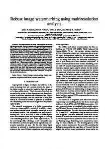
where [.]JC2V2j denotes a sub-sampling by a factor of two in the x and y directions, and where $’ is the optimal prefilter for the cardinal representation. For more details on the specification of the optimal decimation filter, we refer to our previous work14 (cf. Table III, p. 368). The sample values of the spline approximation at scale i will be used to specify the error criterion to be optimized. Also required is the B-spline representation of these signals in order to implement rotations and translations of the reference image r, and to evaluate the partial derivatives of s for the optimization algorithm. Each level of the corresponding B-spline pyramid is obtained by digital filtering of the corresponding sampled representation: c,(k,Z) = (b$
164
“si”(k,Z),
(22)
where (b;)-’ d enotes the impulse response of the so-called direct B-spline filter. The most efficient way to perform this filtering is to use a recursive algorithm lo . Finally, the components of the corresponding image gradient are evaluated by convolution with the appropriate masks l3 . A schematic representation of these various B-spline image processing operations is given in Fig. 1. 3.3 Non-linear least squares optimization One iteration of the optimization algorithm can be described as an attempt to find the best parameter increment (Aa, Ae) such that (23) where c* = R-,T_,q represents a rotated and translated version of the reference according to the current parameter estimates. At scale i where the step size is 2i, the discretized form of the error criterion to be minimized is &;(Aa,,Aa,,Ae)
= ~((T,R,,si)(2’k)-
q*(2’k))l,
ks.+
where Ai represents the region of interest in the image. Our optimization procedure uses a slight modification of the standard Levenberg-Marquardt method for non-linear least squares curve fitting. This technique requires the explicit knowledge of the partial derivatives of the function to be optimized. The derivatives that are needed here can be determined as follows
aThRA,Si(X,Y) il Aa, ‘TbRAoSi(X, iI
Aa,
aT,R,&,Y) aA
=
Aa=O,AIbO
Y)
asi(xPY)
asi(xYY>
= Aa=O,AO=O
(25)
---%--
-7
(26)
(27) Aa=O,A0=0
Since we know the values of &i/ax and asi/& at the grid points (c.f. Section 3.2), these formulas can be used directly to calculate the gradient of the criterion to be optimized, as well as a first order approximation of the Hessian matrix. The best current parameter increments (Aa,, Aa,, AO) are then computed using the recommended Marquardt rule7. The alignment parameters are finally updated as in (15), and the reference image is translated and rotated accordingly by resampling its B-spline representation on the appropriate grid. This procedure is iterated until the minimum is reached. Because of the resampling step, the optimization is always performed around the point (AapO, Aa,,=O,A8=0); this constitutes a variation of the standard Marquardt-Levenberg method. The benefit of this approach is a significant reduction in the number of computations because the partial derivatives of the function on the grid points, as well as the Hessian matrix, need only be computed once per scale. Starting at the coarser scale I, the algorithm first mimics a standard steepest descent procedure, and progressively switches to an inverse-Hessian method as the minimum is approached. The transition to the next finer scale (i-l) occurs once convergence has been reached at resolution i. The method then operates in a quasi-Newton mode until it finally reaches the finer level of the pyramid. The advantage of this strategy is that the largest number of iterations is spent during initialization at the coarser scale; all subsequent finer scale updates usually require no more than one or two iterations since the previous solution already provides a very close estimate. The complexity per iteration is @N/4’) where N denotes the total number of pixels in the image.
165
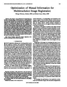
Initialization: Compute the polynomial spline pyramid for the object s and reference r (cf. Fig. la) Initialize (a, 0) For i=I down to 0 Compute the B-spline coefficients for ri and Si (cf. Fig. lb) Compute &J& and a&y at the grid point (cf. Fig. lc) Compute the 3x3 Hessian matrix Repeat Translate and rotate the reference ri according to current estimate (a, 0) Compute the gradient of the error Compute the current error &F(a,8) Compute the Marquardt update for (Au, A@ Update (a, 0) Until convergence End
Fig 2 : Summary of the iterative multiresolution registration procedure. 4. RESULTS 4.1 Cubic spline implementation We used a cubic spline image model (n=3) to implement the algorithm. All the image processing operators described in Section 3.2 are separable; they were implemented by successive one-dimensional processing along the rows and columns. The image translations and rotations were computed by resampling the B-spline expansion (6) at the new pixel locations. Since the basis functions are compactly supported, the image value at a particular location (x, y) is evaluated by partial summation of the B-spline contributions within a local neighborhood. The explicit cubic B-spline formula that was used for this evaluation is 2/3-x2+Ixr/2, p3(x)=
l/3-I&6, I 0,
O