Multisensor Particle Filter Cloud Fusion for Multitarget Tracking Thomas Lang General Dynamics, Ottawa, Canada
[email protected] Michael McDonald DRDC Ottawa, Canada
[email protected]
Daniel Danu, Thia Kirubarajan Department of Electrical and Computer Engineering McMaster University, Hamilton, Canada
[email protected] [email protected] Abstract – Within the area of target tracking particle filters are the subject of consistent research and continuous improvement. The purpose of this paper is to present a novel method of fusing the information from multiple particle filters tracking in a multisensor multitarget scenario. Data considered for fusion is under the form of labeled particle clouds, obtained in the simulation from two probability hypothesis density particle filters. Different ways of data association and fusion are presented, depending on the type of particles used (e.g. before resampling, resampled, of equal or of different cardinalities). A simulation is presented at the end, which shows the improvement possible by using more than one particle filter on a given scenario. Keywords: Tracking, particle filtering, data association, finite random sets.
in local estimators are detailed in section 2. The algorithms for associating and fusing particle clouds (where a cloud is a cluster of particles labeled as pertaining to the same target) generated by two different particle filters are presented in section 3. Ground target tracking simulation and results are given in section 4, while conclusions are drawn in section 5.
2
Because of its ability to handle target birth (or death), track initiation and spawning in a multitarget scenario, the PHD implementation of a particle filter (PHD-PF) was considered for generating particle clouds at local sensor level. Further in this paper sensor and local estimator have a similar meaning, both denoting a local sensor-estimator entity that sends its output data for fusion.
2.1
1
Introduction
Within the last decade and a half, particle filters have been the subject of consistent research and improvements, with special emphasis on target tracking [2]-[10]. The essential work in [2] takes on a single target and, using the bootstrap particle filter, expands tracking performance beyond the classical Extended Kalman Filter (EKF) for nonlinear state dynamics and measurements. In [3] several versions of sampling and resampling developed in the mean-time are presented, while in [4] the authors present an extension of the particle filter to the multitarget case. The fundamental work in [5] on multitarget tracking based on random finite sets (RFSs) and finite set statistics (FISST) derives equations for sequential estimation of the first order multitarget moment aka probability hypothesis density (PHD). Based on the FISST and PHD approaches, new particle filters devised for multitarget scenarios, with the ability to handle target births, deaths and spawning were developed by authors in [6]-[8]. The PHD particle filter was improved in [9]-[10] with track identities, or track labels, use of which is made in the current work during the fusion process. The purpose of this paper is to present a novel method of fusing the information from multiple such particle filters tracking in a multisensor multitarget scenario. Specifics of the particle filters used
Particle Filters
PHD Particle Filter
The PHD definition is based on the theory of RFSs, whose statistics a.k.a. FISST define the targets in a scenario as a RFS (meta-target) and the set of observations as another RFS (meta-observation) [5]. The PHD was introduced in [5] as the first order multitarget moment – the density function whose integral over a region is the expected number of targets in that region. Being defined in singletarget state space, its value at a given point is the probability density function of target presence, therefore provides target localization. In the same work [5] the author derives, within the Bayesian framework of FISST, the sequential estimation of the first order multitarget moment, further known within the target tracking community as the PHD filter. The PHD filter has the ability to initiate tracks of newly born targets, spawning targets, as well as to terminate tracks for dead targets in a multitarget scenario of dynamic target cardinality, while also able to account for clutter within the measurement set. A sequential Monte Carlo implementation of the PHD filter, known as the PHD particle filter, was derived in [6][8].
2.2
Track labeling
One main step of the data fusion process in target tracking is data association, in which data (sets) from different
1191
local estimates are established (grouped) as pertaining to the same target. The fused estimate results from the combination of data contained within such an already associated group (the two steps might overlap or even pass through several iterations in some novel approaches). Data association is a very computationally intensive task, in most cases increasing exponentially with the number of sensors and targets. When fusing particle clouds, the problem is complicated even more, by having for each target a high number of representing particles. This problem is greatly alleviated by labeling particles estimated as representing the same target at the sensor level, prior to fusion. A PHD particle filter with the particle labeling capability was developed in [10]. The main idea is to run in parallel another estimator in order to preserve track identities (e.g. Kalman filter) and associate PHD peaks to current tracks identities. As a result, the PHD particles entering the fusion process, beside the state and weight, have the track label information, which basically them in several herein called clouds. For example, after processing the measurements received at a given time k, the output of a given particle filter s (where s = 1.. S and S is the number of sensors) is the set of labeled
ˆ s, k |k : particles corresponding to the estimated PHD, D
{
}
Dˆ s, k |k = wkls,,sil, ξ kl,s,sil , ls = 1.. Nˆ s, k |k, ils = 1.. Llss, k
combined associated data. Data to be fused here consists of labelled particles and their corresponding weights. The two stages are treated separately next, in developing the fusion method for two sensors.
3.1
Using notations in (1) with time index dropped, we denote by Ξ11 a l1-labeled cloud at sensor one, and by l
l2 = 1.. Nˆ 2 . (We assume that on both sensors labels l1 , l2 are contiguous and start from 1 only for the purpose of
(
simplifying the notation). We denote by cost Ξ11, Ξ 22 l
l
)
the cost of the hypothesis that clouds Ξ11 and Ξ 22 correspond to the same target. Similarly to the case of track-to-track association, if we assume that the cloud association events among different cloud pairs are independent, the most likely cloud-to-cloud association hypothesis can be found, within the 2D1 assignment formulation, by solving the following constrained optimization: l
L1
(
L2
min χ l1l2 cost Ξ11, Ξ 22 χ ∑∑ l1 = 0 l2 = 0
l
l
)
l
(2)
(1) subject to L1
∑χ
l ,i
ls = 1.. Nˆ s, k |k are all targets labels (numbered here from 1 l to Nˆ s, k |k , though this is seldom possible), and Lss, k is the number of particles in the cloud corresponding to track labeled ls, all at time k and at sensor s. In further notation the time index k is dropped for simplification, as fusion is performed statically (at a common instance, thus time being irrelevant for this paper purpose). One advantage of using labeled particles in the particle filter sequential estimation is that new particles can be thrown into processing at any frame around every measurement (true or false) and no estimation of false measurements spatial distribution is needed for generating these new particles. The particles corresponding to false measurements are eliminated in the next frames, as they will not generate usually confirmed tracks, and particles of non-confirmed tracks are not propagated for more than two or three frames. (False tracks, when generated, are usually of small duration.) The advantage of using labeled particles for fusion is that particles of non-confirmed tracks do not enter the fusion process, thus decreasing a lot the data association problem size and communication.
l1l2
l1 = 0
is its weight, Nˆ s, k |k is the estimated number of targets,
3
Ξ l22 a l2-
labeled cloud at sensor two, with labels l1 = 1.. Nˆ 1 and
Here ξ k,ss l is a particle of track label ls and index i, wks, sl l ,i
Association of particle clouds
L2
∑χ
l1l2
l2 = 0
= 1, l2 = 1.. L2
= 1, l1 = 1.. L1
(3)
where χ l1l2 is a binary variable. The labels l1 =0 and l2 =0 in (2-3) are used to denote the association with dummy (therefore no association for the cloud on the other sensor). The minimization in (2)-(3) can be easily solved using for example auction algorithms [12]-[13]. It remains to determine the evaluation of the cloud-to-cloud
(
)
association cost, cost Ξ11, Ξ 22 , which is treated in the l
l
next section. In computing the cloud-to-cloud association cost, two types of clouds are considered (from the particle resampling viewpoint): clouds of unresampled particles and clouds of resampled particles. A gating between clouds has to be used first, such that some costly multiassignments (defined next) are skipped.
3.2
Cost of cloud to cloud association
A particle cloud is a finite set of particles, therefore the cost of associating two clouds can be seen as the distance
Fusion of labeled particle clouds
The fusion part is divided into two main stages, the first being the data association and second the estimation from
1
The optimization problem generalizes to N-D assignment when the number of sensors S > 2.
1192
between the two sets (of M1 and M2 particles) defining the clouds. Prior to computing the cost of associating two clouds
{
Ξ s = ws, ξ s i
i
}
Ms
i =1
, s = 1, 2
Ms
δ Ξ (ξ) = ∑ wsi ⋅ δ ξ (ξ s), s = 1, 2 i =1
(4)
and h(x,y) is defined as M1 M 2
h(x, y) = ∑∑ wijδ ξ1i(x)δ ξ2j (y)
on two sensors (labeled clouds, however, with label dropped here for notation simplification), both clouds are normalized such that their weights sum to one. This is done because we wish to re-interpret the particle cloud as a discretized representation of the target’s probability density function in 2D-Cartesian space, of which integral is one:
∫
dA⊂ R
ps (x, y) ⋅ dA(x, y) = 1
where wij are elements of the transportation matrix W known under this name from the linear programming special case of transportation problem. Introducing (8.1) and (8.2) in (7), the Wasserstein distance applied to two particle clouds becomes:
(5)
d p (Ξ1, Ξ 2) = inf W W
surface area (for estimation in xy plane). A cloud is sent for fusion only if its track was confirmed, therefore the target is almost surely present and (5) holds over the estimation surface R. For the normalized weights we have Ms
∑ ws = ∑ i
i =1
i =1
From (6), upon normalization each particle weight corresponds to the pdf of the cell surrounding the particle (of area ΔA(ξ s) around ξ s ) multiplied by the area cell i
3.2.1
d
W p
s
p
h
M1
∑w
ij
δ Ξ2(ξ 2) , defined on the surfaces ξ s = {(x, y)} , covered by both sensors s = 1, 2 and with values on the discrete sets corresponding to the two particle clouds
{
Ξ1 = ξ ,..., ξ 1 1
M1 1
}
{
, Ξ 2 = ξ ,..., ξ 1 2
M2 2
i =1
(7)
The inclusion of state velocity component into particle distance could be added (i.e. as d = ||x1-x2|| + ε ||v1-v2||) with ε having a the physical meaning small time interval. In [11] the multitarget miss distance is introduced based on the Wasserstein distance as a means to assess the multitarget tracking performance (through providing a distance between the set of estimated tracks and true targets). Here we use the adjustment of Wasserstein distance to finite sets as suggested in [11], the difference being that instead of being applied to sets of targets, it is applied to sets of weighted particles. We use for functions f and g the sum of Dirac delta functions δ Ξ1(ξ1) and
i
p
(9)
j
1 Ms ∑ δξ i(ξ s), s = 1, 2 M s i =1 s
(10)
In this case the transportation matrix W, has the sums on all rows equal, and the same holds for columns:
and
p
ij
i =1 j =1
Using clouds of resampled particles
δ Ξ (ξ) =
mass. The Wasserstein distance defines the dissimilarity between two probability densities f, g, using the distance d (e.g. Euclidian for the case of particles here) and the joint distribution h(x, y) whose marginals are the two densities
∫ h(x, y)dy = f(x) [11]: ( f, g ) = inf ∫ d(x, y) h(x, y)dxdy
∑∑ w d(ξ , ξ )
Using clouds of (labeled) resampled particles at the particle filter level produces a fixed number of particles per cloud, all having same weight (i.e. 1/M for M particles per cloud). The constant weight of all particles results in the special form of δ Ξ s(ξ) as
wsi = psi(ξ si) ⋅ ΔA(ξ si) , representing the cell probability
∫ h(x, y)dx = g(y)
M1 M 2
p
with p = 1 or p = 2. Different methods for computing the cost based on (9) are derived further, depending on the type of particles used (i.e. resampled or before resampling).
Ms wsi i i i A ps (ξ s) ⋅ ΔA(ξ s) = 1 (6) Δ ( ξ ) = s ∑ ΔA(ξ si) i =1
i
(8.2)
i =1 j =1
where R is the region over which the density is estimated, ps is the density function and dA is the elementary
Ms
(8.1)
i s
s
=
1 , M2
M2
∑w
ij
j =1
=
1 M1
(11)
Equations (9) and (11) represent the constrained optimization to be solved in estimating the distance between the clouds (objective function). Two sub-cases arise in the computation of this cost: when Ξ1 = Ξ 2 (i.e. clouds are of equal cardinalities) and when Ξ1 ≠ Ξ 2 .
3.2.1.1 Resampled particle clouds of equal cardinalities For equal cardinalities, M1 = M2 = M and all particles in both clouds have identical weights 1/M. Consequently the cloud-to-cloud association cost can be simplified to the optimal objective function of a simple 2-D assignment (i.e. W to have elements in {0, 1} only). The minimization (9) becomes p d p (Ξ1, Ξ 2) = min σ W
}
1193
1 M
M
∑ d(ξ ,ξσ ) i
i =1
i
p
(12)
with p = 1, 2, where σi is a permutation of i = 1, …, M. Equation (12) represents the 2-D assignment problem (without dummy association allowed, as all particles should be assigned), which can be solved by finding optimum σi permutation using auction algorithms [12][13].
M1
∑w i =1
M2
∑w
ij
j =1
3.2.1.2 Resampled particle clouds of different cardinalities
(14)
= w1, i = 1.. M 1
(15)
i
Constraints (14) and (15) assure that each particle in both clouds is fully assigned (using its full weight) to particles from the other cloud. The minimization problem (13)-(15) is a multiassignment problem, similar to the transportation problem, which is a special case of linear programming.
For clouds of different cardinalities, M 1 ≠ M 2 , even though particles in each cloud have equal weights (i.e. 1/M1 for s = 1 and 1/M2 for s = 2), they are different than particles weights in the other cloud. In order to reduce this problem to a similar 2-D problem as in 3.2.1.1, both clouds need to be reduced to the same number of particles and of equal weights (in order to allow one-to-one associations only and therefore W with elements in {0,1}). Using a method similar to the one in [11], each particle i = 1 .. M1 in the cloud Ξ1 will be resampled into
3.3
Multiassignment solution using linear programming interior point methods
In order to translate (13)-(15) in a classical linear program
subject to
M = M 2 / gcd(M 1, M 2) new particles, where gcd stands * 1
for the greatest common divisor, thus obtaining a cloud of
| Ξ1 | = M 1*M 1 = M 1M 2 / gcd(M 1, M 2) particles of weights w = gcd(M 1, M 2) /(M 1M 2) . The same is done to the particles in the cloud Ξ 2 , in consequence obtaining
we
use
the
min dT w
(16)
Aw = b, w ≥ 0, w ≤1
(17)
following
d∈R
for
M1M 2
,w∈R
M1M 2
,
M1 + M 2
M 1 + M 2, M 1M 2
A∈R ,b ∈ R : d = [d11 d12 ... d1M 2 d 21 d 22 ... d 2M 2 ... d M11 d M12 ... d M1M 2]
| Ξ 2 | = M 2*M 2 = M 1M 2 / gcd(M 1, M 2) particles of same weight w . At this stage the cost can be computed
(
following the same method in 3.2.1.1.
3.2.2
= w2, j = 1.. M 2 j
ij
)
represents the vector of distances d ij = d ξ1 , ξ 2 , i
j
Using clouds of unresampled particles w = [w11 w12 ... w1M 2 w21 w22 ... w2M 2 ... wM11 wM12 ... wM1M 2]T
For two given particle filters s = 1, 2, with M1, respectively M2 total particles per filter at a given time instance, the unresampled particles
{w , ξ } i s
i s
Ms
i =1
is the content of transportation matrix W in vector form,
have
A = [1 1 ... 1 0 0 ... 0 ... 0 0 ... 0 1 0 ... 0 0 1 ... 0 ... 0 0 ... 1
unequal weights. By its nature, for the PHD-PF, the total sum of particles weights is equal to the estimated number Ms
of targets (rational number before rounding)
∑w i =1
i s
= Nˆ s .
For the labeled particle filter, the number of targets is also given (integer) by the number of labels, with only the labels of confirmed tracks counted. A labeled track is considered confirmed only if it has measurements associated to it in several consecutive frames. Only these particles, labeled as pertaining to confirmed tracks, are propagated for fusion. The cost of associating any two clouds is computed as: M1 M 2
(
cost(Ξ1, Ξ 2) = min p ∑∑ wijd ξ1 , ξ 2 i =1 j =1
satisfying the constraints
i
j
)
0 0 ... 0 1 1 ... 1 ... 0 0 ... 0 1 0 ... 0 0 1 ... 0 ... 0 0 ... 1
... 0 0 ... 0 ... 0 0 ... 0 ... ... 1 1 ... 1 ... 1 0... 0 ... 0 1... 0 ... ... 0 0... 1]
(18)
and b = [w1 w2 ... wM1 w1 w2 ... wM 2] being the vector of particle weights of both clouds. 1
1
1
2
2
2
T
A sample package solving the above minimization is LIPSOL (Linear-programming interior point solver) [14].
(13)
3.4
Multiassignment solution as sequential 2D associations
For clouds with very high particle counts, a suboptimal way of performing the multiassignment between
1194
unresampled clouds of different cardinalities is as a sequence of 2D unweighted assignments.
3.5
Cloud to cloud fusion
For two associated particle clouds (as corresponding to same target), Ξ1 and Ξ 2 , of unresampled particles with normalized weights (each cloud weights sum to one), three methods for computing the estimated fused state are presented below. Method 1 – Derives from a direct combination of particles in both clouds, as below
⎛ M1 i i M 2 j j ⎞ xˆ = 0.5 ⎜ ∑ ξ1 w1 + ∑ ξ 2 w2 ⎟ j =1 ⎝ i =1 ⎠
(19) Figure 1 Targets evolution in time in the x, y directions.
Method 2 – Clouds are weighted by their sample covariances, following the information filter approach [1]:
(
−1 −1 xˆ = P1 + P2
)
−1
M2 ⎛ −1 M1 i i j j⎞ −2 ⎜ P1 ∑ ξ1 w1 + P2 ∑ ξ 2 w2 ⎟ (20) i =1 j =1 ⎝ ⎠
where P1 , P2 , are sample covariances of clouds Ξ1 and
Ξ 2 , computed through: Ms
(
)(
Ps = ∑ ws ξ s − ξ s ξ s − ξ s i
i =1
i
i
)
T
, s = 1,2
(21)
where ξ s is the sample weighted mean. In this method independence of the estimation errors of both clouds is assumed. Method 3 – Fusion is carried out making use of the estimated sample cross-covariance matrices between clouds, P12, P21. These are estimated based on the transportation matrix W between clouds, derived in the association step
(
M1 M 2
)(
P12 = ∑∑ wij ξ1 − ξ1 ξ 2 − ξ 2 i =1 j =1 M1
(
= ∑ ξ1 − ξ1 i =1
i
i
)∑ ( M2
j =1
j
)
Figure 2 Targets and measurements in xy plane for the entire scenario simulation.
T
)
T
ξ 2j − ξ 2 wij
(22)
and used as
P = P1 + P2 − P12 − P21
(23)
in the computation of fused estimate N1
N2
i =1
j =1
i i j j −1 −1 xˆ = ( P2 − P21 ) P ∑ ξ1 w1 + ( P1 − P12 ) P ∑ ξ 2 w2 (24)
4
Simulation
The simulation scenario contains several targets which occur and disappear at different moments, as shown through trajectories in Figure 1 below.
Figure 2 shows the true measurements (circles) and false alarms (crosses). The two local estimators used at the two sensors s = 1, 2, are PHD particle filters with track-valued (labeled) particle clouds. The equations and implementation of the track-labelled PHD particle filter follow the one in [10], here extended to two-dimensional tracking, briefly described below, with k denoting the time sample, and filter index s dropped. Particle states contain two-dimensional position and velocity in Cartesian coordinates, while measurements provide only position information. Initialization For i = 1, …, L1 sample position (x, y) of particles as
ξ1,(i x, y) ∼ N ( Z1, σ Z ) , where Z1 is the set of all initial
measurements, and N stands for normal distribution. The velocity components of each particle are initialized uniformly distributed within maximum velocities allowed for a target ξ1,(vx, vy) ∼ U ( −vmax, vmax ) , with vmax = 6 here. i
Initial weights are computed as w1 = ς 1 ( L1 ⋅ n1 ) , where i
1195
ς 1 is the estimated number of targets and n1 is the number
wk = wk |k −1 ⋅ ⎡ β1PDh(z | ξ ki |k −1) β 2PDh(z | ξ ki |k −1) ⎤ P − + + 1 D ⎢ ⎥ ∑ ∑ z∈Z k,in λ ⋅ c + β1Ck (z) z∈Z k,out λ ⋅ c + β 2Ck (z) ⎦ ⎣ i
of measurements. Prediction For i = 1, …, Lk-1 (confirmed particles at time k-1),
(
sample ξ ∼ q ⋅ | ξ i k
i k −1
(27)
) , where q is the proposal density,
which translates into
⎡1 ξ = ⎢⎢00 ⎢⎣ 0 i k
T 1 0 0
0⎤ 0 ⎥ξ i + ν T ⎥ k −1 k 1 ⎥⎦
0 0 1 0
i
(25)
where PD is the probability of detection (considered unity here), h is the sensor measurement function, considered as normal with standard deviation 2.5 for both sensors, λ = 4 is the average rate of clutter points per scan, c = 0.000025 is the uniform clutter density for the whole surveyed area, β1=1.1, β2 = β1/25 are design parameters as in [10] and Lk
Ck(z) = ∑ PDh(z | ξ k |k −1)wk |k −1
with ν k denoting the process noise (vx,y = 1.0, vvx, vy = 0.5) and T = 1 the sampling time step. Assuming no target
i
i
(28)
i =1
spawning, weights are computed as wk = wk −1 ⋅ e , where e = 0.95 is the probability of target survival. For i = Lk-1+1, …, Lk-1+Jk newborn particles are sampled based on new measurements in the set Zk. For this purpose Zk is partitioned with respect to ϒ k −1 , the set of tracks at time k-1, into i
i
{
Z k, in = zkj | zkj in validation region of a track in ϒ k −1 and
}
{
Z k, out = zkj | zkj in no validation region of any track in ϒ k −1
}
Particles position components are sampled for all measurements as ξ k,(x, y) ∼ N ( z,σ z ) , where σz is the i
standard deviation of measurement position error. For measurements in Zk,in particles velocity components are
(
Figure 3 Estimation of single PHD-PF at end of scenario with short false tracks visible. Clouds at current (last) time step: predicted of non-confirmed tracks – blue, current measurements – yellow, confirmed tracks – other color.
)
i n n sampled from ξ k,(vx,vy) ∼ N xˆ k −1,σ v , where xˆ k −1 is the
velocity estimate of track n at time k-1, in which region the measurement z was accepted. For measurements in Zk,out particles velocity components are sampled uniformly within [-vxmax, vxmax] and [-vymax, vymax]. The weights of all newborn particles are computed as
wk |k −1 =
( )
where bk ξ k
i
( ) ⋅ p (ξ | Z ) bk ξ ki
i
Jk
k
i k
(26)
k
is the intensity function of the point
process (considered Poisson here) generating the target birth
and
(
pk ξ ki | Z k
)
the
proposal
density.
By
considering normal densities for bk and pk as in [8],[10] the weights are computed as I / Jk, where the constant intensity of the point process was taken as I = 0.2 (e.g. one target birth expected every 5th sampling time on average). Update For i = 1, …, Lk, where Lk = Lk-1 + Jk, the updated weights are computed as
Figure 4 Estimation results: red, violet – local filters (PHD-PF), blue –true trajectories, cyan – fusion method 1, black – fusion method 2. False tracks eliminated after association are not shown in locally estimated tracks.
Track labels are obtained by using shadow Kalman filters and the resolution cell technique [10]. The unresampled particle clouds are considered for fusion, for which association costs are computed as in (9) with p = 1. RMSE
1196
(Root Mean Square Errors) computed over time for each run and averaged over 100 MC runs are shown in tables below for single filter and fused results. Table 1 RMSE (x, vx, y, vy) for filter 1. RMSE x RMSE vx RMSE y RMSE vy
Target 1
Target 2
Target 3
Target 4
1.7658 2.7756 2.2746 1.1663
1.8079 1.6699 2.0457 1.3235
1.9992 1.8474 1.8778 0.7606
2.0393 1.9771 2.1646 1.2265
Table 2 RMSE (x, vx, y, vy) for Method 1 of fusion RMSE x RMSE vx RMSE y RMSE vy
Target 1
Target 2
Target 3
Target 4
1.3192 2.6851 1.4959 1.1812
1.3582 1.5078 1.4196 1.1471
1.5353 1.8009 1.2962 0.7752
1.6170 1.8394 1.4832 1.0449
Figure 5 Histograms of cloud-to-cloud distances computed : (a) as sum of weighted distances – brown , and (b) using equation (9) – blue for σ1=1.5, σ2=0.5.
Table 3 RMSE (x, vx, y, vy) for Method 2 of fusion. RMSE x RMSE vx RMSE y RMSE vy
Target 1
Target 2
Target 3
Target 4
1.7658 2.6158 1.5531 1.1109
1.3442 1.4193 1.4254 1.0945
1.5765 1.7308 1.2717 0.7242
1.6273 1.7897 1.4222 1.0013
From results above it can be seen that position estimates are improved more than velocity estimates, and that the usage of sample covariances in Method 2 does not increase consistently the accuracy.
4.1
Monte Carlo simulation for Gaussian distributed clouds
In order to assess the proposed association cost for clouds of different distributions, Monte Carlo simulations were performed for estimating the association cost of two clouds, normally distributed (corresponding to the unresampled case), with different standard deviations. The number of particles considered was M = 200 on both clouds. The cost distributions obtained in 50 runs are compared with the distribution of the distance between the clouds centers estimated using the weighted sum of particles
d12 =
M
M
∑ w ξ −∑ w ξ i =1
i i 1 1
j j 2 2
Figure 6 Same distributions as in Fig. 5, for σ1=1.5, σ2=1.0.
(29)
j =1
From the histograms of the distances computed using (9) and (29), compared in Fig. 5-9 for clouds of different distributions, it can be seen that the cost computed based on (29) is insensitive to the variance of the clouds, as only the first order estimate enters (29), while the one computed based on (9) increases with the difference between clouds standard deviation (variance). While these simulations were using Gaussian clouds, however the cost in (9) is not making any assumption on normality, therefore differences in higher order moments of the clouds are expected to be reflected in the costs as well.
Figure 7 Same distributions as in Fig. 5 for σ1=1.5, σ2=1.5.
1197
[3] Sanjeev M. Arulampalam, S. Maskell, N. Gordon, and T. Clapp, A tutorial on particle filters for online nonlinear/non-Gaussian Bayesian tracking, IEEE Trans. on Signal Processing, Vol 50, No. 2, pp. 174-188, February 2002. [4] Carine Hue, J-P Le Cadre, Patrick Perez, Tracking Multiple Objects with Particle Filtering, IEEE Trans. on AES, Vol. 38, No. 3, pp. 791-812, July 2002. [5] Ronald P.S. Mahler, Multitarget Bayes filtering via first-order multitarget moments, IEEE Trans. on AES, Vol. 39, No. 4, pp. 1152-1178, October 2003. Figure 8 Same distributions as in Figures 5-7, for σ1=1.5, σ2=2.5.
[6] T. Zajic and R. Mahler, A particle-systems implementation of the PHD multitarget tracking filter, Signal Proc., Sensor Fusion and Target Recognition XII, SPIE Proc. I. Kadar (ed.), Vol. 5096, pp. 279-290, 2003. [7] Hedvig Sidenbladh, Multi-target particle filtering for the Probability Hypothesis Density, The 6th International Conference on Information Fusion, Cairns, Australia, July 2003, Proc. Vol.2, pp. 800-806. [8] Ba-Ngu Vo, Sumeetpal Singh, Arnaud Doucet, Sequential Monte Carlo Methods for Multi-Target Filtering with Random Finite Sets, IEEE Trans. on AES, Vol. 41, No. 4, pp. 1224-1245, October 2005.
Figure 9 Same distributions as in Figures 5-7, , for σ1=1.5, σ2=3.5.
5
Conclusion
A method of fusing density estimates of particle filters at the particle cloud level was proposed. Cloud-to-cloud association costs depending on particles types were developed together with several fusion methods. Results obtained for a simulated multitarget scenario of dynamic cardinality were presented. The fusion at particle level results in a fused estimate of target density, not only in a fused estimate of the target state; the improvement of the target density estimate will be further investigated.
References
[9] K. Panta, B. Vo, S. Singh, Improved probability hypothesis density (PHD) filter for multitarget tracking, The 3rd Conf. on Intelligent Sensing and Information Processing, Bangalore, India, December 2005, Proc. pp. 213-218. [10] Lin Lin, Yaakov Bar-Shalom, T. Kirubarajan, Track labeling and PHD filter for multitarget tracking, IEEE Trans. on AES, Vol. 42, No. 3, pp. 778-794, July 2006. [11] John R. Hoffman and Ronald P. S. Mahler, Multitarget Miss Distance via Optimal Assignment, IEEE Trans. on Systems, Man and Cybernetics - Part A Systems and Humans, Vol. 34, No. 5, May 2004. [12] Dimitri P. Bertsekas, and David A. Castañon, A forward/reverse auction algorithm for asymmetric assignment problem, Technical Report Lids-P-2159, MIT, 1993.
[1] Y. Bar-Shalom, X.R. Li, T. Kirubarajan, Estimation with Applications to Tracking and Navigation: Theory, Algorithms and Software, Wiley, New York, 2001.
[13] R. Jonker and A. Volgenant, A shortest augmenting path algorithm for dense and sparse linear assignment problems, J. Computing, Vol. 38, pp. 325-340, 1987.
[2] Neil. J. Gordon, D.J. Salmond, and A.F.M. Smith, Novel approach to nonlinear/non-Gaussian Bayesian state estimation, IEE Proceedings-F Radar, Sonar and Navigation, Vol. 140, No. 2, pp. 107-113, April 1993.
[14] Yin Zhang, User’s guide to LIPSOL linearprogramming interior point solvers v0.4, Optimization Methods and Software, Vol. 11-12, pp. 385-396, 1999.
1198