Nerve Cell Segmentation via Multi-Scale Gradient Watershed Hierarchies Yi-Ying Wang, Yung-Nien Sun, Chou-Ching K. Lin and Ming-Shaung Ju Abstract - Automated segmentation of nerve cell in microscopic image is an important task in neural researches. We proposed a multi-scale watershed-based approach to cope with this microscopic image analysis problem. There are three stages in the proposed segmentation algorithm: (1) a multi-scale watershed scheme is used to estimate an initial location of nerve cell nuclei; (2) we can identity nerve cell nuclei according to properties of nerve cell and watershed results in different scale; (3) Once the possible nerve cell is identified as a true one, a fuzzy rule based Active Contour Model (ACM) is applied to find the optimal outer contour. Our approach can segment nerve cell automatically and accurately. The cell detection rates in the experiments are above 95%. Moreover, the fuzzy rule based ACM provides flexible alternative to handle cell contour detection.
I. INTRODUCTION ERVE fiber detection is an essential task to extract important biological features in neural researches. However, there are hundreds of axons in each nerve which make manual measurements difficult to conduct. In the past few years, there have been several studies presented on neural cell segmentation. By simply threshold method or canny edge [1], we have found that it is hardly possible to outline regions of interest in microscopic image. The main problem is that the retained edges are mostly disconnected. In [2], a multi-stage segmentation method based on compact Hough transform (CHT) is applied to determine the possible locations of cell nuclei. A likelihood function was then defined to optimize the cell boundary. In [3], all axon centers were first roughly estimated by elliptical Hough transform. Then cell boundaries were refined by ACM. Other references can be found in [4-6]. However, the number of detected axons is relatively small in these studies [1-6]. In this paper, we proposed a new segmentation method that detects a large amount of axons by watershed algorithm and then extracts outer boundaries of axons by applying ACM based on fuzzy rules.
N
Manuscript received April 24, 2006. This work was supported by the Taiwan
National
Science
Council
under
contract
NSC94-2614-E-006-075. Y. N. Sun and Y. Y. Wang are with Department of Computer Science and Information Engineering; Chou-Ching K. Lin is with Department of Neurology; Ming-Shaung Ju is with Department of Mechanical Engineering, National Cheng Kung University, Tainan, Taiwan, R.O.C. (corresponding author: Yung-Nien Sun; phone: +886 -2757575-62526; fax:+886-2747076;e-mail:
[email protected])
II. MATERIALS AND METHODS The cross-sectional images of nerve cell were first acquired from microscopes that are equipped at the National Cheng Kung University Hospital, Tainan, Taiwan. The RGB images were transformed to an 8-bit gray-scale image using equation (1).
g = 0.33 × red + 0.5 × green + 0.17 × blue ,
(1)
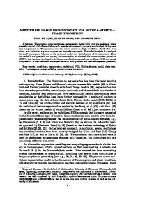
where red, green, blue are intensities (0 - 255) of red, green and blue channels in color image, and g is the gray-scale intensity. A typical cross sectional nerve image was given in Fig. 1 (a). In general, the intensity of cell nuclei is brighter than the myelin sheath. Myelin sheath is the ring area enclosed by inner and outer contours, in which the intensity is lower than cell nucleus. Thus, we generally define a cell as a nucleus surrounded by myelin sheath as in Fig.1 (b). We introduce the nerve cell segmentation process as follows: 1) First step – multi-scale watershed segmentation: We first extend the morphological watershed algorithm by Vincent and Soille [7] to a multi-scale hierarchy for segmenting the cell boundaries. The proposed algorithm was applied to overcome two problems which are poor image quality or local variations of cells and difficulty to examine all cells using single scale. For example, if the contrast between cells and background is large, we can find these cells in the coast scale. In the contrary, if the intensity of cells is weak or not clear, it may only be shown in the finest one. For multi-scale watershed segmentation, we can build a multi-scale gradient watershed hierarchy scheme which can adapt to different scale for all cell nuclei detection. 2) Second step – identification of cell nuclei: After multi-scale watershed segmentation procedure, we can obtain an estimate location of each cell nuclei. Double checking the watershed region was necessary to verify if a real cell was correctly located because the detected region may be an interstice between cells. We used the property of cells (as in Fig 1 (b)) to identify the falsely-detected axons. 3) Third step – ACM based on fuzzy rules In general, ACM has the difficulty in defining suitable weights in its energy function. To overcome this problem, the proposed ACM defines the energy function based on fuzzy rules can perform contour deformation more flexibly. In. [8-9], the other ACM with fuzzy rules is used and achieve better results. After the region of cell
nucleus was appropriately identified in the second step, we apply the new ACM based on fuzzy rules to determine its outer boundary. Different to [8-9], we proposed to use a grid search to find the optimal solution. III. NUCLEI CELL SEGMENTATION PROCEDURE In this section, we describe the proposed algorithm for cell segmentation in detail. A. Multi-Scale Watershed Segmentation At first, the gradient magnitude image was computed and used as input image of watershed transform to obtain the watershed lines. Multi-scale watershed segmentation is achieved by sequentially changing the immersion levels in implementing watershed transform. We first define the notations in multi-scale watershed transform. Assign p = {R , R ,..., R } to be the initial partition of image at the coast scale after applying the gradient watershed transform. In order to demonstrate the watershed segmentation result at each scale, the hierarchical scale m is defined as m } . The relationship between scales m and p m = {R1m , R2m ,...Rnm m m −1 m-1 is p ⊆ p , which means that each segment in p m is one to one mapping to the one in p m −1 . Let Sim−1 be a segmented region i at scale m-1, and this area maps onto the image at scale m and obtains bim corresponding regions. We can then check the homogeneity of Sim−1 based on these bim disjoint regions. Fig.2 shows different immersion level l results in different region numbers. The smaller l is, the larger the region number. The relationship between immersion level l and scale m is illustrated in Fig. 2 (b) to (h). 1
1 1
1 2
1 n1
B. Identification of Cell Nuclei By using a multi-scale watershed segmentation procedure in section III A, an approximate region is segmented for each possible cell nucleus. However, not all segmented regions can be confirmed as true cell nuclei. Thus, the second step is to identify the real cells. We use the following conditions to reconfirm whether the segmented regions are cells. Condition (1): The watershed region r has not been marked in the previous scale m-1. Condition (2): The region r is mapped to the finest scale M. If region r has brM mapping regions in the finest scale, we then calculate the individual mean intensity for each of the brM mapping regions. If the difference between maximal and minimal mean intensity of these brM regions is less than Tint , the region r is regarded as a homogenous one. Condition (3): Compute the largest and shortest distance of region r from its center to boundary. If the ratio of largest to shortest length is less then Tdis , region r forms a circular (or elliptic) shape. Condition (4): The mean intensity of region r is larger than
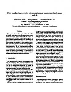
that of its surrounded regions. If a region r obeys these four conditions, we regard it as a cell nucleus. C. ACM Based on Fuzzy Rules After confirming all cell nuclei, the detected cell contour, typically as in Fig. 3(a), is used as an initial estimate to find the outer boundary by applying ACM based on Fuzzy Rules. The candidate boundary points are estimated by the following steps: 1) N equally spaced nodes are sampled from the initial contour and denoted as w(1), w(2), …w(N). 2) Each search line i is defined to be perpendicular to the line segment connecting w(i-1) and w(i+1). 3) H grid points centered at the initial node w(i) are chosen along the search line i. Fig.3 shows candidate nodes in the grid search. Here, we define v(i, j ) is the jth node located in the ith search line. The fuzzy ACM is then applied to every node v(i, j ) . The fuzzy degree at every node v(i, j ) is denoted as μ (v(i, j )) which is estimated by using the following information: 1) Smoothness: The first feature value, S, is to estimate the smoothness of contour at selected node v(i, j ) and is given as follows:
⎛ | v′(i, j ) |2 + | v′′(i, j ) |2 ⎞ , (2) S = 1 − min⎜⎜ , 1⎟⎟ sm ⎝ ⎠ where v′(i, j ) is the first derivative and represents continuity, v′′(i, j ) is the second derivative and represents curvature and sm is a scaling factor. When the contour at node v(i, j ) is smooth, S has high value. 2) Circular (or elliptic) shape: The second feature is D that represents the circular or elliptic shape.
D=
min(d min , d cur ) , max(d max , d cur )
(3)
where d max and d min are the farthest and nearest Euclidean distances from the initial contour nodes to the center of initial contour. d max and d min are updated at each iteration. d cur is the Euclidean distance between the current node v(i, j ) and the center of the initial contour. In general, the larger the D is, the more circular the shape is. 3) Maximal gradient magnitude:
G=
Δg i , g max − g min
(4)
where Δg i = g (i, j + 1) − g (i, j ) , g(i, j +1) and g (i, j ) are gray levels at the j+1th and jth grid points on search line i, G is the corresponding normalized magnitude, and gmax and gmin are the maximal and minimal gradient values located on the search line, respectively. The third feature G is in fact a
normalized gradient. After the three features are obtained at node v(i, j ) , we can compute fuzzy degree μ (v(i, j )) according to fuzzy rules listed in Table I. The fuzzy linguistic rules are used to map the three features into the output space. Fuzzy rules can effectively represent the experience of an expert [10]. The structure of a rule is given as follows: Rule: If Premise Then Conclusion, where the premise is linked by fuzzy operator ∧ (AND). Low, Median and High are the linguistic values of membership function illustrated in Fig. 4. A Min-Max technique developed by Mamdani et al. [10] is adopted to implement the fuzzy rules. Fuzzy rules are then applied to every node v(i, j ) and the mean fuzzy degree is computed using equation (5). N
μ contour = (1 / N )∑ μ (i) ,
(5)
i =1
where μ (i) is equal to the maximal of μ (v(i, j )) along the search line i and N is the number of nodes along the cell contour. The procedure of maximizing the fuzzy rules based ACM is implemented as follows: Let C0 (w0 (1), w0 (2), w0 (3),..., w0 ( N )) be the initial positions of nodes on the initial curve C0 . The following steps are employed in the optimization process at the k-th iteration. Step (1): For a node wk (i ) on curve Ck , for all the candidate nodes v(i, j ) on the search line i, calculate the three feature values. Step (2): Estimate fuzzy degree μ (v(i, j )) at every node v(i, j ) . Step (3): Find μ (i) which is equal to the maximal of μ (v(i, j )) along the search line i and then move node wk (i ) to v(i, j ) at which the fuzzy degree is maximal. Step (4): Apply Step 1-3 to all nodes on every search line. k +1 Compute the fuzzy degree, μ contour , which belongs to the curve Ck +1 (wk +1 (1), wk +1 (2), wk +1 (3),..., wk +1 ( N )) . Step (5): If μ is not larger than the previous fuzzy k degree, μcontour , the procedure is terminated. After finishing the iterative procedure, the outer boundaries are detected. Then, a spline interpolation is applied to obtain a continuous contour. The whole cell nerve segmentation procedure can be summarized as follows: Step (1): Multi-scale gradient watershed segmentation is executed to obtain initial cell contours at all scales. Step (2): At the current scale, check every region if it conforms the cell properties. Step (3): If the region is a cell nucleus then do fuzzy ACM. Step (4): Scale+1, then go to step (2), until the finest scale.
immersion level l is from 1 to 30. Without loss of generality, the cells too close to the image boundary and the cells with nucleus areas less than ten pixels were ignored in performance evaluation. And each test image was rotated by 0°、90°、180°、and 270°. The average performance, including average FP、average FN and average detection rate, are calculated by averaging the results from the four different angles. Our average detection rate is about 97% (142/146 and 136.3/141 as shown in Table II). From the average performance, we can declare that our cell segmentation method is robust and has high performance. V. CONCLUSION The proposed method for neural cell detection consists of three steps: detection of possible nuclei via multi-scale watershed segmentation, cell reconfirmation, and outer contour optimization by fuzzy ACM. The major difficulty in manual assessment of nerve cells is to handle the huge amount of axons in neural image. By applying the flexibility in multi-scale watershed and the knowledge embedded in fuzzy rule based ACM, we can successfully handle the complication in automated cell segmentation. In experiments, we have applied the method to several images and obtained encouraging results.
B
A (a) (b) Fig.1. (a) A typical nerve-cell image. Size of image is 256×256. (b) An enlarged nerve cell. Arrows A and B point to cell nucleus and myelin sheath respectively.
k +1 contour
Tint
IV. EXPERIMENTAL RESULTS In the experiments, we have chosen seven parameters = 20, Tdis = 5, sm = 100, N = 12, H = 10, M = 30 and
(a)
(b)
(c)
(d)
(e) (f) (g) (h) Fig.2. Segmented results with different immersion level l. (a) Original image. From (b) to (h), immersion level l= 1, 2, 3, 4, 5, 6, 7 and correspond to scale m = 7, 6, 5, 4, 3, 2, 1 with 342, 317, 296, 276, 266, 249 and 232 regions.
.. .
..
. i=3
j=1 j=H
i=2 i=1
i=N
(a) (b) Fig.3 Illustration of the grid search. (a) A segment of inner contour from watershed segmentation. (b) There are N search lines. Each search line contains H grid points.
Low
Fuzzy Degree
1
Median
High
Feature 0
0.25
0.50 0.75
1.0
Fig.4. Fuzzy membership functions.
TABLE I. FUZZY RULES USED TO DETECT CELL CONTOUR Rule 1: If (S is L ) ∧ (D is L ) ∧ (G is L) Then (μ is L ) Rule 2: If (S is M) ∧ (D is L) ∧ (G is L ) Then (μ is L) Rule 3: If (S is H ) ∧ (D is L) ∧ (G is L ) Then (μ is L) Rule 4: If (S is L ) ∧ (D is L ) ∧ (G is M) Then (μ is L) Rule 5: If (S is M) ∧ (D is L) ∧ (G is M) Then (μ is L) Rule 6: If (S is H ) ∧ (D is L) ∧ (G is M) Then (μ is M) Rule 7: If (S is L ) ∧ (D is L) ∧ (G is H ) Then (μ is L ) Rule 8: If (S is M) ∧ (D is L) ∧ (G is H ) Then (μ is M) Rule 9: If (S is H ) ∧ (D is L) ∧ (G is H ) Then (μ is M) Rule 10: If (S is L ) ∧ (D is M) ∧ (G is L) Then (μ is L) Rule 11: If (S is M) ∧ (D is M) ∧ (G is L) Then (μ is L) Rule 12: If (S is H ) ∧ (D is M) ∧ (G is L) Then (μ is M) Rule 13: If (S is L ) ∧ (D is M) ∧ (G is M) Then (μ is L) Rule 14: If (S is M) ∧ (D is M) ∧ (G is M) Then (μ is M) Rule 15: If (S is H ) ∧ (D is M) ∧ (G is M) Then (μ is M) Rule 16: If (S is L ) ∧ (D is M) ∧ (G is H) Then (μ is M) Rule 17: If (S is M) ∧ (D is M) ∧ (G is H) Then (μ is M) Rule 18: If (S is H) ∧ (D is M) ∧ (G is H) Then (μ is L ) Rule 19: If (S is L ) ∧ (D is H) ∧ (G is L ) Then (μ is L ) Rule 20: If (S is M) ∧ (D is H) ∧ (G is L ) Then (μ is M ) Rule 21: If (S is H ) ∧ (D is H) ∧ (G is L ) Then (μ is M ) Rule 22: If (S is L ) ∧ (D is H) ∧ (G is M) Then (μ is M) Rule 23: If (S is M) ∧ (D is H) ∧ (G is M) Then (μ is M) Rule 24: If (S is H ) ∧ (D is H) ∧ (G is M) Then (μ is H) Rule 25: If (S is L ) ∧ (D is H) ∧ (G is H ) Then (μ is M ) Rule 26: If (S is M) ∧ (D is H) ∧ (G is H ) Then (μ is H) Rule 27: If (S is H ) ∧ (D is H) ∧ (G is H ) Then (μ is H) L=LOW, M=MEDIAN, H=HIGH.
Fig.5 (a) Original image.
(b) Segmentation result.
TABLE II. PERFORMANCE OF CELL DETECTION ALGORITHM Image # of avg. # of Avg. Avg. Avg. Avg. det. ID det. cell true cell FP FN TP rate (%) Fig.5 146.8 146 4.75 4 142 97.3 Fig.6 140.3 141 3.8 4.3 136.3 96.7 FP = False Positive is defined as the total number of detected cells that do not exist in reality. FN = False Negative is defined as the total number of cells that exist in reality but are discarded by the detection procedure. TP = False Positive is defined as the total number of detected cells that exist in
Fig.6 (a) Original image.
(b) Segmentation result.
REFERENCE [1] P. Mussio, et.al., “Automatic cell count in digital images of liver tissue sections,” 4th IEEE Symp. on CBMS, pp. 153-160, 1991. [2] Y.L. Fok, J. C. K. Chan, and R. T. Chin, “Automated Analysis of Nerve-Cell Images Using Active Contour Models,” IEEE Trans. on Medical Imaging, vol. 15, no. 3, pp. 353-368, 1996. [3] T. Mouroutis, S.J. Roberts and A.A. Bharath, “Robust cell nuclei segmentation using statistical modeling,” Bioimaging, vol. 6, no. 2, pp. 79-91, 1998. [4] C. D. Ruberto, A. Dempster, S. Khan, and Bill Jarra, “Analysis of infected blood cell images using morphological operators,” Image and Vision Computing, vol. 20, no. 2, pp. 133-146, 2002. [5] P. Bamford, and B. Lovell, “Unsupervised cell nucleus segmentation with active contours,” Signal Processing, vol. 71, no. 2, pp. 203-213, 1998.
reality. Detection rate = (TP)/ (# of true cell). [6] J. AF Costa, ND Mascarenhas, and ML De Andrade Netto, “Cell nuclei segmentation in noisy images using morphological watersheds,” Proc. SPIE vol. 3164, pp. 314-324, 1997. [7] L Vincent, P Soille, “Watersheds in Digital Spaces: An Efficient Algorithm Based on Immersion Simulations,” IEEE Trans. on Pattern Analysis and Machine Intelligence, vol. 13, no.6, pp.583-598, 1991. [8] K Syoji, F Yuji, et.al. “Interactive segmentation of the cerebral lobes with fuzzy inference in 3T MR images,” IEEE Trans. on Systems, Man and Cybernetics, Part B, vol. 36, no. 1, pp.74-86, 2006. [9] W. Abd-Almageed, A. El-Osery, and C. E. Smith, “A Fuzzy-Statistical Contour Model for MRI Segmentation and Target Tracking,” Proc. of SPIE vol. 5438, pp.25-33. [10] E. H. Mamdani and S. Assilian, “An experiment in linguistic synthesis with a fuzzy logic controller,” Int. J. Man-Mach. Stud., vol. 7, no. 1, pp. 1-13, 1975.