Networked Control Systems: A Model-Based Approach - CiteSeerX

The Handbook of Networked and Embedded Systems Hristu and Levine, Eds. pp. 601-626, Birkhauser, 2005.

Networked Control Systems: A Model-Based Approach Luis A. Montestruque, Panos J. Antsaklis University of Notre Dame, Notre Dame, IN 46556, U.S.A. {lmontest, pantsakl}@nd.edu

Key words: control over networks, stabilizability, minimum feedback information, model-based control Summary. In this article a class of networked control systems called Model-Based Networked Control Systems (MB-NCS) is considered. This control architecture uses an explicit model of the plant in order to reduce the network traffic while attempting to prevent excessive performance degradation. MB-NCS can successfully address several important control issues in an intuitive and transparent way. In this article the main results of this MB approach are described with examples. Specifically, conditions for the stability of state and output feedback continuous and discrete systems are derived under different scenarios that include delay compensation, constant and time varying update times, non-linear plants and quantization of the feedback signals. In addition, a performance measure for MB-NCS with noise inputs is introduced.

1 Introduction A networked control system (NCS) is a control system in which a data network is used as feedback medium. NCS is an important research area; see for example [16] and [15, 18, 19]. The use of networks as media to interconnect the different components in an industrial control system is rapidly increasing. The use of networked control systems poses, though, some challenges. One of the main problems to be addressed when considering a networked control system is the size of the bandwidth required by each subsystem. It is clear that the reduction of bandwidth necessitated by the communication network in a networked control system is a major concern. This can perhaps be addressed by two methods: the first method is to minimize the transfer of information between the sensor and the controller/actuator; the second method is to compress or reduce the size of the data transferred at each transaction. Since

2

Luis A. Montestruque, Panos J. Antsaklis

shared characteristics among popular industrial networks are small transport time and big overhead, using less bits per packet has small impact on the overall bit rate. So reducing the rate at which packets are transmitted brings better benefits than data compression in terms of bit rate used. In this paper, we consider the problem of reducing the packet rate of a NCS using a novel approach called Model-Based NCS (MB-NCS). The MB-NCS architecture makes explicit use of knowledge about the plant dynamics to enhance the performance of the system. Model-Based Networked Control Systems (MBNCS) were introduced in [11]. In Section 2 the basic MB-NCS setup is introduced for continuous plants. Stability of MB-NCS’ with no quantization and periodic transmissions are considered. In Section 3 a performance measure is introduced for the previously presented MB-NCS. The stability of MB-NCS with time-varying and stochastic transmission times is studied in Section 4. Quantization schemes are considered in Section 5. Finally, stability for a class of nonlinear systems is studied in Section 6.

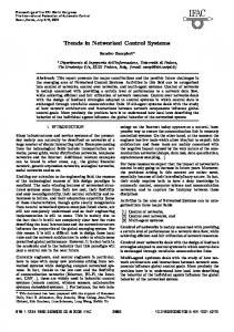
2 Stability of Continuous Linear MB-NCS with Constant Update Times 2.1 State Feedback MB-NCS We consider the control of a continuous linear plant where the state sensor is connected to a linear controller/actuator via a network. In this case, the controller uses an explicit model of the plant that approximates the plant dynamics and makes possible the stabilization of the plant even under slow network conditions.

Fig. 1. Proposed configuration of networked control system.

We will concentrate on characterizing the transfer time between the sensor and the controller/actuator, which is the time between information exchanges.

Networked Control Systems: A Model-Based Approach

3

The plant model is used at the controller/actuator side to recreate the plant behavior so that the sensor can delay sending data since the model can provide an approximation of the plant dynamics. The main idea is to perform the feedback by updating the model’s state using the actual state of the plant that is provided by the sensor. The rest of the time the control action is based on a plant model that is incorporated in the controller/actuator and is running open loop for a period of h seconds. The control architecture is shown in Figure 1. Our approach is novel in that it incorporates a model of the plant, the state of which is updated at discrete intervals by the plant’s state. We present a necessary and sufficient condition for stability that results in a maximum transfer time. We make use of standard stability definition such as the ones found in [1]. If information for all the states is available, then the sensors can send this information through the network to update the model’s vector state. For our analysis we will assume that the compensated model is stable and that the transportation delay is negligible. We will assume that the frequency at which the network updates the state in the controller is constant. The idea is to find the smallest frequency at which the network must update the state in the controller, that is, an upper bound for h, the update time. Usual assumptions in the literature include requiring a stable plant or in the case of a discrete controller, a smaller update time than the sampling time. Here we do not make any of these assumptions and the plant may be unstable. Consider the control system of Figure 1 where plant is given by x˙ = Ax + ˆx + Bu, ˆ and the controller by u = K x Bu, the plant model by x ˆ˙ = Aˆ ˆ. The state error is defined as e = x − x ˆ, and represents the difference between the plant state and the model state. The modeling error matrices A˜ = A − Aˆ and ˜ = B −B ˆ represent the difference between the plant and the model. We will B £ ¤T now express the combined state z(t) = x(t)T e(t)T in terms of the initial condition x(t0 ). A necessary and sufficient condition for · stability of the state ¸ A + BK −BK feedback MB-NCS will then be presented. Define Λ = ˜ ˜ . ˜ A + BK Aˆ − BK Proposition 1 [13] The State Feedback MB-NCS with initial conditions £ ¤T z(t0 ) = x(t0 )T 0T = z0 , has the following response: Λ(t−tk )

z(t) = e

µ·

¸ · ¸¶k I 0 Λh I 0 e z0 , 00 00

for t ∈ [tk , tk+1 ), with tk+1 − tk = h Theorem 1 [13] The State Feedback MB-NCS is globally exponentially stable £ T T ¤T around = 0 if and only if the eigenvalues of · the¸ solution · ¸z = x e I 0 Λh I 0 M= e are strictly inside the unit circle. 00 00

4


One can gain insight into the · closed¸ loop·system ¸ behavior by noticing that I 0 Λh I 0 the nonzero eigenvalues of M = are exactly the eigenvalues e 00 00 of another matrix: ˆ

ˆ

N = e(A+BK)h + eAh

Z

h

ˆ BK)τ ˆ (A+ ˜ e−Aτ (A˜ + BK)e dτ

(1)

0

This can be shown either directly or by using the Laplace transform. The second method involves replacing the update time variable h by the time variable t, transforming the expression using the Laplace transform. The transformed expression can then be easily manipulated. After isolating the upper left block matrix, inverse Laplace transform can be used to return to time domain [10]. First we observe that the eigenvalues of the compensated model apRh pear in the first term of N . We can see the term ∆ = eAh 0 e−Aτ (A˜ + ˆ BK)τ ˆ (A+ ˜ BK)e dτ as a perturbation on the desired eigenvalues, that is, the eigenvalues of the compensated model. Even if the eigenvalues of the original plant were unstable the perturbation ∆ can be made small enough by having ˜ small and thus minimizing their impact over the eigenvalues of h and A˜ + BK the compensated plant. We also observe that if the update time h is driven to zero, then ∆ = 0. Also it is possible to make ∆ = 0 by having a plant model that is exact. Example 1 Consider the following unstable plant (double integrator): A = · ¸ · ¸ 0 1 0 , B= We will use the state feedback controller given by u = Kx 0 0 £ 1 ¤ with K = −1 −2 . Usually it is assumed that the actuator/controller will hold the last value received from the sensor until the next time the sensor transmits and a packet is received. Under this assumption the controller/actuator’s model acts as a zero order hold when updated. We will first analyze this situation. To do so, we will transform the plant model so that it holds the last state ˆx + Bu ˆ , with update to it by the network. This is given by: x ˆ˙ = Aˆ · presented ¸ £ ¤ 0 0 ˆ = 0 0 T . Now we need to search for the biggest h such Aˆ = and B 0 0 · · ¸ ¸ I 0 Λh I 0 that e has its eigenvalues inside the unit circle. To do so we 00 00 plotted the maximum eigenvalue magnitude versus the update time. The plot is shown in Figure 2. From Figure 2 we see that the condition for stability is to have h < 1 second. In fact the test matrix M will have one eigenvalue with magnitude 1 for h = 1 second and the system will be marginally stable. If we use the results by [19] we would have obtained that, in order to stabilize the system, we would need to have h < 2.1304 × 10−4 seconds, which is very conservative. Simulations of the system with update times of 2.1304 × 10−4 and 0.5 seconds


5

are shown in Figure 3. Note that the plant was initialized with an initial £ ¤T condition of 1 1 . max eigenvalue magnitude

2.5

2

1.5

1

0.5 0

0.5

1

1.5

update times h

Fig. 2. Maximum eigenvalue magnitude of the test matrix M versus the update time h.

h=0.5 sec 1.5

1

1 plant state

plant state

h=0.0002 sec 1.5

0.5 0

−0.5 −1

0.5 0

−0.5

0

5

time (sec)

10

15

−1

0

5

time (sec)

10

15

Fig. 3. System response for h = 2.1304 × 10−4 and h = 0.5 sec.

It is clear that the performance obtained with h = 0.5 seconds is not too different to the one obtained with h < 2.1304×10−4 seconds, but the difference in the amount of bandwidth used is large. If we were to use Ethernet that has a minimum message size of 72bytes (including preamble bits and start of delimiter fields) the data rate would be 2.7Mbits/sec for the case of h < 2.1304 × 10−4 seconds, and 1.2Kbits/sec for the case of h = 0.5 seconds. Example 2 In real applications uncertainties can frequently be expressed as tolerances over the different measured parameter values of the plant. This can be mapped into structured or parametric uncertainties on the state space matrices. Next an example is given on how the Theorem 1 can be applied if two entries on the A matrix of the model can vary within a certain interval.

6


· ¸ · ¸ 0 1 ˆ= 0 ; Aˆ = ,B 1 ¸ · ¸ ·0 0 0 0 1+a ˜12 ; ,B= plant: A= 1 0+a ˜21 0 with a ˜12 =£ [−0.5, 0.5], ˜21 = [−0.5, 0.5] ¤ a controller: K = −1 −2 . model:

The system will now be tested for an update time of h = 2.5 seconds. The following contour plot in Figure 4 represents the magnitude of the maximum eigenvalue of the test matrix M as a function of the (1,2) and (2,1) entries of A parameters a12 and a21 . Here the contour of height equal to one is the relevant one to stability. It is easy to isolate the stable and unstable regions in the uncertainty parameter plane. The stable region is between the lines labeled as 1.

1

1.6

0.2

1

0.2 0.4

0.4

0.8

0.6

1.4 1.2

0.3

2 1.8

0.4

0.6 0.8

0.5

0.2

0.8 1

0.2

0.4

0.

6

2

0.6

0.4

0. 0.

a21

2

1.4

1.2

0

1.8

8

0.1

1.6

−0.1

0.

0.2

0.8

0.6

2 0.

−0.5 −0.5

−0.4

−0.3

−0.2

−0.1

0

0.1

0.2

1.6

1

0.

4

1.2

1.4

−0.4

1.8

−0.3

4

−0.2

0.3

0.4

0.5

a

12

Fig. 4. Contour Plot Maximum Eigenvalue Magnitude vs Model Error.

2.2 Output Feedback MB-NCS We have been considering plants where the full state vector is available at the output. We now extend our approach to include plants where the state is not directly measurable. In this case, in order to obtain an estimate of the plant state vector, a state observer is used. It is assumed that the state observer is ˆx + Bu, ˆ to collocated with the sensor. Again, we use the plant model, x ˆ˙ = Aˆ design the state observer. The observer uses the plant output and generates a copy of the plant input applied by the controller. See Figure 5. Having the sensor carry the computational load of an observer is justified by the fact that typically sensors that can be connected to a network have an embedded processor inside. This processor is usually in charge of performing the sampling, filtering and implementing the network layer services required to connect to the network. Ishii and Francis give a similar justification in


7

Fig. 5. Proposed configuration of an output feedback networked control system.

[17]. In their approach an observer is placed at the output of the plant to reconstruct the state vector. The result is then quantized and sent over the network to the controller. The observer has as inputs the output and input of the plant. In the implementation of this set up, to acquire the input of the plant, which is at the other side of the communication link, the observer can have a version of the model and controller, and knowledge of the update time h. In this way, the output of the controller, that is the input of the plant, can be simultaneously and continuously generated at both ends of the feedback path with the only requirement that the observer makes sure that the model has been updated. This last requirement ensures that both the controller and the observer are synchronized. Handshaking provided by most network protocols can be used. ˆx + Bu, ˆ to design the state observer. Again, we use the plant model, x ˆ˙ = Aˆ See Figure 5. The observer has the form of a standard state observer with gain L. In summary, the system dynamic equations are for t ∈ [tk , tk+1 ): Plant: Model: Controller: Observer:

x˙ = Ax + Bu, y = Cx + Du ˆx + Bu, ˆ y = Cˆ x ˆ x ˆ˙ = Aˆ ˆ + Du u = Kx ˆ £ ¤£ ¤ ˆ x+ B ˆ − LD ˆ L uT y T T x ¯˙ = (Aˆ − LC)¯

We now proceed in a similar way as in the previous case of full feedback. There will be an update interval h, after which the observer updates the controller’s model state x ˆ with its estimate x ¯. Define an error e that will be the difference between the controller’s model state and the observer’s estimate: e = x ¯−x ˆ. Also define the modeling error matrices in the same way as before: A˜ = A− Aˆ , £ ¤T ˜ =B−B ˆ , C˜ = C − Cˆ , and D ˜ = D − D. ˆ Define z = xT x ¯T eT , and B  A BK −BK ˆ + LDK ˜ −BK ˆ − LDK ˜  Λo =  LC Aˆ − LCˆ + BK ˜ ˆ ˆ ˜ LC LDK − LC A − LDK 

8


Theorem 2 [13] The Output Feedback MB-NCS is globally exponentially sta£ T T T ¤T ¯ e ble around = 0 if and only if the eigenvalues  the solution  z = x x I00 I00 of Mo =  0 I 0  eΛo h  0 I 0  are inside the unit circle. 000 000

The eigenvalues of the test matrix Mo can be studied in a similar fashion as in the state feedback case. By replacing h by t, applying the Laplace transform and isolating the nonzero upper left block of Mo we obtain: ³ ´−1 ³ ´−1  −1 ˆ − BK ˆ ˆ ˆ sI − A + ∆ (sI − A) BK sI − A − BK 1   ³ ´−1 P =  sI − Aˆ + LCˆ ∆3 + ∆2

with ˜ ˆ −1 ∆1 = (sI − A)−1 (A˜ + BK)(sI −³ Aˆ − BK) ´ ´ ³ ˆ −1 ˆ −1 BK ˜ − A˜ − LC˜ (sI − A)−1 BK (sI − Aˆ − BK) ∆2 = (sI − Aˆ + LC) ´ ´´ ³ ³ ³ ˜ ˆ −1 A˜ − LC˜ + BK ˜ − A˜ − LC˜ (sI − A)−1 A˜ + BK · ∆3 = (sI − Aˆ + LC) −1 ˆ ˆ (sI − A − BK)

˜ → 0 , and C˜ → 0 then ∆1 → 0 , ∆2 → 0 , and It is clear that if A˜ → 0 , B ∆3 → 0. By doing so we obtain: ³ ³ ´−1  ´−1 −1 ˆ ˆ ˆ ˆ (sI − A) BK sI − A − BK   sI − A − BK ³ ´−1 PL = lim P =   ∆→0 ˆ ˆ 0 sI − A + LC

From here it can be seen that by making the error between the plant and thenmodel zero, compensated eigenvalues would be placed at o o the system’s n ˆ ˆ ˆ BK)h ˆ (A−L C)h (A+ . Similarly to the full state feedback case, ∪ eig e eig e there are perturbation matrices ∆1 , ∆2 , and ∆3 that can be made small by reducing the error between the actual plant and the model dynamic equations. The perturbation is over a matrix that has the eigenvalues of the compensated model. Finally note that the separation principle of classic control where controller and observer can be designed independently cannot be used here. 2.3 State Feedback MB-NCS with Network Induced Delays Previously we assumed that the network delays were negligible. This is usually true for plants with slow dynamics relative to the network bandwidth. When this is not the case the network delay cannot be neglected. Network delays can occur for many reasons. There are three important delay sources: • •

Processing time. Media access contention.


•

9

Propagation and transmission time.

The first one, processing time, occurs at both ends of the communication channel. On the transmitter, the processing time is the time elapsed between the time the transmitting process makes the request to the operating system to transmit a message, to the time the message is ready to be sent. And on the receiver this is the time interval that occurs between the last bit of the message is received by the receiver, and when the time the message is delivered by the operating system to the receiver process. The media access contention time is the time the transmitter has to wait until the communication channel is not busy. This is usually the case when several transmitters have to share the same media. The propagation and transmission time is the time the message takes to be placed on the network media and to travel through the network to reach the receiver. In local area networks the time the message takes to travel or propagate through the media is small in comparison to wide area networks or internetworks like the Internet. The time the message takes to be placed on the network depends on the size of the message and the baud rate. If the control network is a local area network, as is common practice in industry, the propagation and transmission time can be established beforehand with good accuracy. Similarly for the processing time. If real time operating systems are used the processing time can be accurately calculated. Finally, media access contention delay can be fixed with the use of a communication protocol with scheduling. Fast data communication networks like Token Ring, Token Bus, and ArcNet fall into this category. Industry oriented control networks like Foundation Fieldbus also implements a scheduler through its LAS or Link Active Scheduler. Even the inherently non-deterministic Ethernet has addressed the problem of not having a specified contention time with the so-called Switched Ethernet. In conclusion, most of these delays can at least be bounded if the network conditions are appropriate. In the following, we extend our results to include the case were transmission delay is present. We will assume that the update time h is larger than the delay time τ . As before we will assume that the update time h and delay τ are constant. We will present here the case of full state feedback systems. So, at times kh − τ the sensor transmits the state data to the controller/actuator. This data will arrive τ seconds later. Therefore, at times kh the controller/actuator receives the state vector value x (kh − τ ). The main idea is to use the plant model in the controller/actuator to calculate the present value of the state. After this, the state approximate obtained can be used to update the controller’s model as in previous setups. The system is depicted in Figure 6. The Propagation Unit uses the plant model and the past values of the control input u(t) to calculate an estimate of actual state x ˘(kh) from the

10


Fig. 6. Proposed configuration of a state feedback networked control system in the presence of network delays .

received data x(kh − τ ). This estimate is then used to update the model that with the controller will generate the control signal for the plant. The system is described by the following equations: Plant: x˙ = Ax + Bu ˆx + Bu ˆ Model: x ˆ˙ = Aˆ Controller: u = Kx ˆ, t ∈ [tk , tk+1 ) ˆx + Bu, ˆ t ∈ [tk+1 − τ, tk+1 ] Propagation Unit: x ˘˙ = A˘ Update law: x ˘ ← x, t = tk+1 − τ and x ˆ←x ˘, t = tk+1

(2)

We define the errors eˆ = x ˘−x ˆ and e˘ = x − x ˘. We also make the following definitions:     A + BK −BK −BK x A˜ = A − Aˆ ˜ Aˆ − BK ˜ −BK ˜  , z =  e˘   A˜ + BK , Λ = d ˜ =B−B ˆ B eˆ 0 0 Aˆ Theorem 3 [13] The State Feedback MB-NCS with networked induced delay £ ¤T τ is globally exponentially stable around the z = xT e˘T eˆT =0   solution I00 I00 if and only if the eigenvalues of MT =  0 I 0  eΛd τ  0 0 0  eΛT (h−τ ) are 0II 000 inside the unit circle. It is interesting to note that the results on Theorem 3 can be seen as a generalization of Theorem 1. This can be shown by driving τ to zero. Example 3 Here we ·present ¸ a numeric · ¸ example with the same plant we have 0 1 0 been using before A = ,B= , with randomly generated plant model 0 0 1


·

¸

·

11

¸

£ ¤ −0.3444 0.9225 ˆ = −0.0098 , and controller K = −1 −2 . , B −0.3089 0.3560 1.3159 Figure 7 shows the plots for the maximum eigenvalue magnitude as a function of h for 3 different values of τ . The maximum value h can have to preserve stability is reduced when τ is increased.

Aˆ =

1.15

max eigenvalue magnitude

1.1

1.05

1

0.95

0.9

0.85

0.8 0.5

0.6

0.7

0.8

0.9

1

1.1

1.2

1.3

1.4

1.5

update times h

Fig. 7. Maximum eigenvalue of test matrix M versus the update times h for τ = 0, 0.25, and 0.50 sec.

3 A Performance Index for Linear MB-NCS with Constant Update Times The performance characterization of Networked Control Systems under different conditions is also of mayor concern together with stability. It is clear that, since the MB-NCS is h-periodic, there is no transfer function in the normal sense whose H2 norm can be calculated [2]. For LTI systems the H2 norm can be computed by obtaining the 2-norm of the impulse response of the system. We will extend this definition to specify an H2 norm, or more accurately, to define an H2-like performance index [2]. We will call this performance index Extended H2 Norm. We will study the Extended H2 Norm of the MB-NCS with output feedback studied in subsection 2.2. A disturbance signal w and a performance or objective signal z are included in the setup. We will start by defining the system dynamics: Plant Dynamics: x˙ = Ax + B1 w + B2 u z = C1 x + D12 u y = C2 x + D21 w + D22 u

Define the following:

Observer Dynamics: ˆ2 − LD ˆ 22 )u + Ly x ¯˙ = (Aˆ − LCˆ2 )¯ x + (B Model Dynamics: ˆx + B ˆ2 u x ˆ˙ = Aˆ Controller: u = Kx ˆ

(3)

12


 A B2 K −B2 K ˆ2 K + LD ˜ 22 K −B ˆ2 K − LD ˜ 22 K  Λ =  LC2 Aˆ − LCˆ2 + B ˜ ˆ ˆ ˜ LC2 LD22 K − LC2 A − LD22 K     I00 B1 £ ¤ M (h) =  0 I 0  eΛh , BN =  LD21  , CN = C1 D12 K −D12 K 000 LD21 

Theorem 4 [21] The Extended H2 Norm, kGkxh2 , of the Output ¢ ¡ TFeedback MB-NCS described in Equation (3) is given by kGkxh2 = trace BN XBN where X is the solution of the discrete Lyapunov equation M (h)T XM (h) − X + Wo (0, h) = 0 and Wo (0, h) is the observability Gramian computed as Rh T T Wo (0, h) = 0 eΛ t CN CN eΛt dt. Note that the observability Gramian can be factorized as Caux T Caux = T T eΛ t CN CN eΛt dt. This allows one to compute the Extended Norm as the 0 regular H2 norm of a discrete LTI system. Rh T T CN eΛt dt and the auxiliary Corollary 1 [21] Define Caux T Caux = 0 eΛ t CN discrete system Gaux with parameters Aaux = M (h), Baux = BN , Caux , and Daux = 0, then the following holds. Rh

kGkxh2 = kGaux k2 Example 4 We now present an example using a double ¸ ¸ integrator ·as the · 0.1 0 1 , , B1 = plant. Let the plant dynamics be given by: A = 0.1 0 0 £ ¤T £ ¤ £ ¤ B2 = 0 1 , C1 = 0.1 0.1 , C2 = 1 0 , D11 = 0 , D12 £ = 0.1¤, D21 = 0.1 , D22 = 0 . We will use the state feedback controller K = −1 −2 . £ ¤T A state estimator with gain L = 20 100 is used to place the state observer eigenvalues· at –10. We will use the following parame¸ a plant · model with ¸ £ ¤ 0.1634 0.8957 −0.1686 ˆ ˆ ˆ ters: A = , B2 = , C2 = 0.8764 0.1375 , −0.1072 −0.1801 1.0563 ˆ 22 = −0.1304 . D In Figure 8 we plot the extended H2 norm of the system as a function of the updates times. Note that as the update time of the MB-NCS approaches zero, the value of the Extended H2 norm approaches the H2 norm of the nonnetworked compensated system. Also note the performance degradation as the update time h is increased.

4 Stability of MB-NCS with Time-Varying Update Times In this section we relax our assumption that the update times h(k) are constant. Here we study the state feedback MB-NCS shown in Figure 1. The


13

0.045 0.04 0.035

0.0394

zw

||G ||

2 xh2

0.03 0.025 0.02 0.015 0.01 0.005 0 0

1

2

3

4

5

6

update times h (sec)

Fig. 8. Extended H2 norm of the system as a function of the update times.

packets transmitted by the sensor contain the measured value of the plant state and are used to update the plant model on the actuator/controller node. These packets are transmitted at times tk . We define the update times as the times between transmissions or model updates: h(k) = tk+1 − tk . Previously we made the assumption that the update times h(k) are constant. This might not always be the case in applications. The transmission times of data packets from the plant output to the controller/actuator might not be completely periodic due to network contention and the usual non-deterministic nature of the transmitter task execution scheduler. Soft real time constraints provide a way to enforce the execution of tasks in the transmitter microprocessor. This allows the task of periodically transmitting the plant information to the controller/actuator to be executed at times tk that can vary according to certain probability distribution function. This translates into an update time h(k) that can acquire a certain value according to a probability distribution function. Most work on networked control systems assumes deterministic communication rates [17,20] or time-varying rates without considering the stochastic behavior of these rates [9, 19]. Little work has concentrated in characterizing stability or performance on a networked control system under time-varying, stochastic communication. We first study the stability properties of the feedback MB-NCS assuming that the update times can take any values in an interval [hmin , hmax ]. In this case we will assume that we don’t have any statistical knowledge about the update times. We analyze the stability properties of this system using Lyapunov techniques. This is the strongest type of stability presented and will provide a first cut on the characterization of the stability properties perhaps for comparison purposes. Next, two types of stochastic stability are discussed, namely Almost Sure or Probability-1 Asymptotic Stability and Mean Square or Quadratic Asymptotic. The first one is the one that mostly resembles deterministic stability [3]. Mean square stability is attractive since it is related to optimal control problems such as the LQR.

14


Two different types of time-varying transmission times are considered for each case of stochastic stability criterion. The first assumes that the transmission times are independent identically distributed with probability distribution function that may have support for infinite update times. The second type of stochastic update time assumes that the transmission times are driven by a finite Markov chain. Both models are common ways of representing the behavior of network transmission and scheduler execution times. 4.1 Lyapunov Stability of MB-NCS The stability criterion derived in this section is the strongest and most conservative stability criterion. It is based on the well-known Lyapunov second method for determining the stability of a system. We will assume that the properties of h(k) are unknown but h(k) is contained within some interval. This criterion is not stochastic but provides a first approach to stability for time-varying transmission times NCS. Definition 1 The equilibrium z = 0 of a system described by z˙ = f (t, z) with initial condition z(t0 ) = z0 is Lyapunov asymptotically stable at large (or globally) if for any ε > 0 there exists β > 0 such that the solution of z˙ = f (t, z) satisfies kz (t, z0 , t0 )k < ε , ∀t > t0 and lim kz (t, z0 , t0 )k = 0 t→∞

whenever kz0 k < β. Theorem 5 [14] The State Feedback MB-NCS is Lyapunov Asymptotically Stable for h ∈ [hmin , hmax ] if there exists a symmetric positive definite matrix T X such that· Q = is positive definite for all h ∈ [hmin , hmax ] ¸ ¸ X −· M XM I 0 Λh I 0 . where M = e 00 00 Theorem 5 may be used to derive an interval [hmin , hmax ] for h for which stability is guaranteed. It is clear that the range for h, that is the interval [hmin , hmax ], will vary with the choice of X. Another observation is that the interval obtained this way will always be contained in the set of constant update times for which the system is stable (as derived using Theorem 1). That is, an update time contained in the interval [hmin , hmax ] will always be a stable constant update time. Several ways of obtaining the values for hmin and hmax can be used. One is to first fix the value of Q, obtain the solution X of the Lyapunov equation in Theorem 5 for a value of h known to be stable. Then, using this value of X, the expression X − M XM T can be evaluated for positive definiteness. This can be repeated for all the values of h known to stabilize the system to obtain the widest interval [hmin , hmax ]. 4.2 Almost Sure or Probability-1 Asymptotic Stability We will use the definition of almost sure asymptotic stability [3] that provides a stability criterion based on the sample path. This stability definition


15

resembles more the deterministic stability definition [4], and is of practical importance. Since the stability condition has been relaxed, we expect to see less conservative results than those obtained using the Lyapunov stability considered in the previous section. We now define Almost Sure or Probability-1 Asymptotic stability. Definition 2 The equilibrium z = 0 of a system described by z˙ = f (t, z) with initial condition z(t0 ) = z0 is almost sure (or with probability-1) asymptotically stable at large (or globally) if for any β > ¾ 0 and ε > 0 the solution of ½ z˙ = f (t, z) satisfies lim P

sup kz (t, z0 , t0 )k > ε

δ→∞

= 0 whenever kz0 k < β.

t≥δ

This definition is similar to the one presented for deterministic systems in Definition 1. We will examine the conditions under which the full state feedback continuous networked system in Figure 1 is stable. MB-NCS with Independent Identically Distributed Transmission Times Here we will assume that the update times h(k) are independent identically distributed (iid) with probability distribution function F (h). We now present the conditions under which the full state feedback MB-NCS with iid update times is asymptotically stable with probability-1. We will use a technique similar to lifting [2] to obtain a discrete linear time invariant representation of the system. It can be observed that the system can be described by ξk+1 = Ωk ξk , with ξk ∈ L2e and ξk = z(t + tk ), t ∈ [0, hk ).

(4)

Here L2e stands for the extended L2 . It can be shown that the operator Ωk can be represented as: Λt

(Ωk ν)(t) = e

·

I0 00

¸ h(k) Z δ(τ − h(k))ν(τ )dτ

(5)

0

With δ(t) representing the impulse function. Now we can restate the definition on almost sure stability or probability-1 stability given in Definition 2 to better fit the equivalent system representation (4). Definition 3 The system represented by (4) is almost sure stable or stable with probability-1( if for any β > 0 and ε ) > 0 the solution of ξk+1 = Ωk ξk satisfies: lim P ˜ δ→∞

sup kξk (t0 , z0 )k2,[0,tk ] > ε k≥δ˜

= 0 whenever kz0 k < β. Where

the norm k·k2,[0,h(k)] is given by kξk k2,[0,h(k)] =

Ã

h(k) R 0

2

kξk (τ )k dτ

!1/2

.

16


This definition allows us to study almost sure stability of systems such as (4) when the probability distribution function for update times has infinite support. Based on this definition the following result can now be shown. Theorem 6 [14] The State Feedback MB-NCS, with update times h(j) independent identically distributed random variable with probability distribution F (h) is globally almost sure (or with probability-1) stable h¡ asymptotically £ T T ¤T ¢1/2 i 2¯ σ (Λ)h around the solution z = x e = 0 if N = E e < ∞ −1 and the expected value of the maximum singular value of· the ¸test matrix · ¸ M, I 0 Λh I 0 E [kM k] = E [¯ σM ], is strictly less than one, where M = . e 00 00 Note that the condition may give conservative results if applied directly over the test matrix. To avoid this problem and make the condition tighter we may apply a similarity transformation over the test matrix M . The condition on the matrix N ensures that the probability distribution function for the update times F (h) assigns smaller occurrence probabilities to increasingly long update times, that is F (h) decays rapidly. In particular we observe that N can always be bounded if there exists hm such that F (h) = 0 for h larger thanhhm . We can alsoi bound the expression inside the expecta¡ ¢1/2 £ ¤ < E eσ¯ (Λ)h and formulate the following tion to obtain E e2¯σ(Λ)h − 1 corollary: Corollary 2 The State Feedback MB-NCS, with update times h(j) that are independent identically distributed random variable with probability distribution F (h) is globally almost sure (or with probability-1) asymptotically sta¤T £ ¤ £ = 0 if T = E eσ¯ (Λ)h < ∞ and ble around the solution z = xT eT the expected value of the maximum singular value of the test matrix M , E [kM k] = E [¯ σM ], is strictly less than one. £ ¤ Note that Corollary 1 condition T = E eσ¯ (Λ)h < ∞ is automatically satisfied if the probability distribution function F (h) doesn’t have infinite support. It otherwise indicates that F (h) should roll off fast enough as to counteract the growth of M ’s maximum singular value as h increases. Example 5 We use the unstable double integrator plant. We now assume that h(k) is a random variable with a uniform probability distribution function U (0.5, hmax ). The plot of the expected maximum singular value of a similarity transformation of the original test matrix M is shown in Figure 9. The similarity transformation used here was one that diagonalizes the matrix M for h = 1. We see that the maximum value for hmax is around 1.3 seconds (maximum constant update time for stability is h = 1 second.) So we see that, the double integrator with uniformly distributed update time between 0.5 and 1.3 seconds is stable, while the same system but with a constant update time of 1 second is unstable. This also represents an improvement over the result that we may


17

have obtained by using the previously discussed Lyapunov Stability condition in which the maximum update time obtainable would have been less than 1sec. 2.2 2

E[||M||] for h~U(0.5,hmax)

1.8 1.6 1.4 1.2 1 0.8 0.6 0.5

1

1.5

2

hmax (sec)

Fig. 9. Average Maximum Singular Value for h ∼ U (0.5, hmax ) as a function of hmax , zero dynamics plant model.

1.2

E[||M||] for h~U(0.5,hmax)

1.1

1

0.9

0.8

0.7

0.6

0.5

1

2

3 4 hmax (seconds)

5

6

Fig. 10. Average Maximum Singular Value for h ∼ U (0.5, hmax ) as a function of hmax , improved plant model.

The advantage of using a model-based approach resides in its ability to reduce the amount of bandwidth required. The previous example shows stability conditions for a model that represents a zero order hold, that is, the control value is kept constant until the next update time. We will now show the same plots for a model that better resembles the plant; this was done by randomly perturbing¸ the plant The plant model matrices are: ¸ · matrices. · 0.0871 0.0844 0.9353 ˆ = . Figure 10 shows that stability is , B Aˆ = 1.0834 0.0476 −0.0189 maintained for update times that have uniform distribution with a max update time of 5.5 seconds. This shows that improved knowledge over the plant dynamics can translate into a significant improvement in terms of stability.

18


MB-NCS with Markov Chain-Driven Transmission Times In certain cases it is appropriate to represent the dynamics of the update times as driven by a Markov chain. A good example of this is when the network experiences traffic congestion or has queues for message forwarding. We now present a stability criterion for the model-based control system in which the update times h(k) are driven by a finite state Markov chain. Assume that the update times can take a value from a finite set: h (k) ∈ {h1 , h2 , ..., hN } and hi 6= ∞, ∀i ∈ [1, N ]

(6)

Let us represent the Markov chain process by {ωk }with state space {1, 2, ..., N } and transition probability matrix Γ and N × N matrix with elements pi,j and ¤T £ initial state probability distribution Π0 = π1 π2 ... πN . The transition probability matrix entries are defined as pi,j = P{ωk+1 = j|ωk = i}. We can now represent the update times more appropriately as h(k) = hωk . A sufficient condition for the almost sure stability of the system under Markovian jumps is given in the following theorem. Theorem 7 [14] The State Feedback MB-NCS with update times h(k) = hωk 6= ∞ driven by a finite state Markov chain{ωk } with state space {1, 2, ..., N } and transition probability matrix Γ with elements pi,j and initial state proba¤T £ is globally almost sure asymptotically bility distribution Π0 = π1 π2 ... πN £ T T ¤T = 0 if the matrix T has all its stable around the solution z = x e eigenvalues inside of the unit circle, where:   0 0 0 kM |h1 k · · ¸ ¸   T 0 kM |h2 k 0 0  Γ ; M |hi = I 0 eΛhi I 0 T =   0 0 ... 0 00 00 0 0 0 kM |hN k If Γ is irreducible it follows that, since kM k is non-negative, T is also irreducible. Then it can be shown using the Perron-Frobenius theorem as in [6], that T ’s maximum magnitude eigenvalue is real and sometimes referred to as the Perron-Frobenius eigenvalue. 4.3 Mean Square or Quadratic Asymptotic Stability We now define a different type of stability, namely Mean Square Asymptotic Stability: Definition 4 The equilibrium z = 0 of a system described by z˙ = f (t, z) with initial condition z(t0 ) = z0 is mean square stable asymptotically stable at ilarge h

(or globally) if the solution of z˙ = f (t, z) satisfies: lim E kz (t, z0 , t0 )k t→∞

2

=0


19

A system that is mean square stable will have the expectation of system states converging to zero with time in the mean square sense. This definition of stability is attractive since many optimal control problems use the squared norm in their formulations. We will study the two cases studied in the previous section under this new stability criterion. MB-NCS with Independently Identical Distributed Transmission Times We present the conditions under which the state feedback networked control system is mean square stable, we also discuss how these conditions relate to the ones for probability-1 stability. Theorem 8 [14] The State Feedback MB-NCS with update times h(j) independent identically distributed random variable with probability distribution F (h) is globally mean square stable around the solution h¡ asymptotically ¢2 i £ ¤T z = xT eT = 0 if K = E eσ¯ (Λ)h < ∞ and the maximum singu° £ T ¤° ¡ £ T ¤¢ °E M M ° = σ lar value of the expected value of ·M T M , ¯ E M M , is · ¸ ¸ I 0 Λh I 0 strictly less than one, where M = e . 00 00 We note the similarity between the conditions given by Theorems 6 and 8. For the first one we require the expectation of the maximum singular value of the test matrix to be less than one. While for the second stability criterion it is required to have the maximum singular value of the expectation of the test matrix (multiplied by its transpose) to be less than one. MB-NCS with Markov Chain-Driven Transmission Times The type of stability criteria above depend on our ability to find appropriate P (i) matrices. Several other results in jump system stability [5, 7] can be extended to obtain other conditions on stability of networked control systems. Note though, that most of the results available in the literature deal with similar but not identical type of systems. Theorem 9 The State Feedback MB-NCS with update times h(k) = hωk 6= ∞ driven by a finite state Markov chain {ωk } with state space {1, 2, ..., N } and transition probability matrix Γ with elements pi,j is globally mean square £ ¤T asymptotically stable around the solution z = xT eT = 0 if there exists positive definite matrices P (1), P (2), . . . , P (N ) such that:   · ¸ N X ¡ ¢ I0  pi,j H(i)T P (j)H(i) − P (i) < 0, ∀i, j = 1..N with H(i) = eΛhi 00 j=1

20


5 Stability of Linear MB-NCS with Quantization Here we extend our stability results to consider the case where quantization errors occur. In particular a state space MB-NCS is considered. Two static quantizers are studied: the Uniform Quantizer and the Logarithmic Quantizer. These are called static since they partition the state space into invariant regions that are fixed in time. We also note that these quantizers represent two of the most common data representations: fixed point format for uniform quantizers and floating point format for logarithmic quantizers. We will assume that the transmission times are constant. We will also assume that the compensated networked system without quantization is stable which in view of Theorem 1 there exists positive definite P that satisfies: ³ ´ ³ ´ T ˆ ˆ ˆ ˆ e(A+BK ) h + ∆(h)T P e(A+BK )h + ∆(h) − P = −QD (7) Rh

ˆ BK)τ ˆ (A+ ˜ BK)e ˜ e−Aτ (A+ dτ and with QD symmetric and ˆ ˆ A+BK )h ( positive symmetric. Note that e +∆ (h) was previously defined in (1).

where ∆(h) = eAh

0

5.1 State Feedback MB-NCS with Uniform Quantization Define the Uniform Quantizer as a function q : Rn → Rn with the following property kz − q(z)k ≤ δ, z ∈ Rn , δ > 0. Theorem 10 [21] The plant state of the State Feedback MB-NCS satisfying (7) and using the Uniform Quantizer will enter and remain in the region kxk ≤ R defined by: ´ ³ ¡ ¢ ˆ ˆ R = eσ¯ (A+BK )h + ∆max (h) r + eσ¯ (A)h + ∆max (h) δ r λmax ((eAh −∆(h))T P (eAh −∆(h))T )δ 2 where r = λmin (QD ) ´ R h σ¯ (A)(h−τ ) ³ ˆ ˆ ˜ and ∆max (h) = 0 e σ ¯ A˜ + BK eσ¯ (A+BK )τ dτ 5.2 State Feedback MB-NCS with Logarithmic Quantization Define the Logarithmic Quantizer as a function q : Rn → Rn with the following property kz − q (z)k ≤ δ kzk , z ∈ Rn , δ > 0. Theorem 11 [21] The State Feedback MB-NCS satisfying (7) and using the Logarithmic Quantizer is exponentially stable if: v u λmin (QD ) u ³ ´ δ 0.

(13)

Theorem 12 [21] The non-linear MB-NCS with dynamics described by (8), that satisfies the Lipschitz conditions described by (12) and with exponentially stable compensated plant model satisfying (13) is asymptotically stable if: µ µ ¶¶¶ µ ¢ K δ ¡ Kf h β 1 − α e−βh + e − e−βh >0 β Kf + β

Theorem 12 presents a sufficient condition for stability of a class of nonlinear systems. Note that if the model has the exact same dynamics as the plant, that is if Kδ = 0, then the condition will be satisfied for arbitrarily large h. Example 7 We use the inverted pendulum in Figure 12 as example.

Fig. 12. Inverted Pendulum.

The parameters for the plant are g = 10, L = 10, k = 0.1, and m = 1.01. The model parameters are the same as the plant ones,£ except for ¤the mass that is m = 1.00. Finally the controller is given by: τ = −316 316 x ˆ. Using the following Lipschitz and exponential stability constants: Kf = 1.0507, Kδ = 0.0450, α = 1.5, and β = 0.6, Theorem 12 predicts stability for update times between 0.55 and 2.55 sec. Simulations show that the system is unstable for h greater that approximately 4.5 sec.


23

Conclusions The MB-NCS control architecture presented in this chapter represents a natural way of placing critical information about the plant on the network so to reduce the data traffic load. By making the sensor and actuator more “intelligent” the networked control system is able to predict the future behavior of the plant, and send the precise information at critical times so to ensure plant stability. Model-based networked control systems are only one of the various approaches to networked control. We study these systems since the benefits and properties they have make them well suited for a variety of practical applications. Furthermore, the control structures presented appear to be amenable to detailed analysis. Acknowledgements The partial support of the Army Research Office (DAAG19-01-1-0743) and of the the National Science Foundation (NSF CCR-02-08537 and ECS-0225265) is gratefully acknowledged.

References 1. P. Antsaklis and A. Michel, “Linear Systems,” McGraw-Hill, New York 1997. 2. T. Chen and B. Francis, “Optimal Sampled-Data Control Systems,” 2nd edition, Springer, London 1996. 3. F. Kozin, “A Survey of Stability of Stochastic Systems,” Automatica Vol5 pp. 95-112, 1968. 4. M. Mariton, “Jump Linear Systems in Automatic Control” Marcel Dekker, New York 1990. 5. O.L.V. Costa and M.D. Fragoso, “Stability Results for Discrete-Time Linear Systems with Markovian jumping Parameters,” Journal of Mathematical Analysis and Applications, Vol 179, pp. 154-178, 1993 6. A. Dembo and O.Zeitouni, “Large Deviation Techniques and Applications,” Springer-Verlag, New York, 1998. 7. Y. Fang, “A New General Sufficient Condition for Almost Sure Stability of Jump Linear Systems,” IEEE Transactions on Automatic Control, Vol 42, No3, pp. 378-382, March 1997. 8. S. Woods, “Probability, Random Processes, and Estimation Theory for Engineers,” 2nd edition, Prentice Hall, Upper Saddle River 1994. 9. A.S. Matveev and A.V. Savkin, “Optimal Control of Networked Systems via Asynchronous Communication Channels with Irregular Delays,” 40th IEEE Conference on Decision and Control, Orlando Florida, December 2001, pp. 2323-2332. 10. L.A. Montestruque and P.J. Antsaklis, “Model-Based Networked Control Systems: Stability,” ISIS Technical Report ISIS-2002-001, University of Notre Dame, www.nd.edu/∼isis/, January 2002. 11. L.A. Montestruque and P.J. Antsaklis, “Model-Based Networked Control Systems: Necessary and Sufficient Conditions for Stability,” 10th Mediterranean Conference On Control And Automation, July 2002.

24


12. L.A. Montestruque and P.J. Antsaklis, “State And Output Feedback Control In Model-Based Networked Control Systems,” 41st IEEE Conference on Decision and Control, December 2002. 13. L.A. Montestruque and P.J. Antsaklis, “On the Model-Based Control of Networked Systems,” Automatica, Vol 39, pp 1837-1843. 14. L.A. Montestruque and P.J. Antsaklis, “Stability of Networked Systems with Time Varying Transmission Times,” Transactions of Automatic Control, 2004, to appear. 15. G.N. Nair and R.J. Evans, “Communication –Limited Stabilization of Linear Systems,” Proceedings of the Conference on Decision and Control, 2000, pp. 10051010. 16. –, Networked Control Sessions, Proceedings of the Conference on Decision and Control, Proceedings of the American Control Conference, 2003. 17. H. Ishii and B. Francis, “Stabilizing a Linear System by Switching Control and Output Feedback with Dwell Time,” Proceedings Of The 40 th IEEE Conference On Decision And Control, December 2001, pp. 191-196. 18. J.K. Yook, D.M. Tilbury, and N.R. Soparkar, “Trading Computation for Bandwidth: Reducing Communication in Distributed Control Systems using State Estimators,” IEEE Transactions on Control Systems Technology, July 2002, Vol 10, No.4, pp. 503-518. 19. G. Walsh, H. Ye, and L. Bushnell, “Stability Analysis of Networked Control Systems,” Proceedings of American Control Conference, June 1999. 20. D. Hristu-Varsakelis, “Feedback Control Systems as Users of a Shared Network: Communication Sequences that Guarantee Stability,” Proceedings of the 40 th IEEE Conference on Decision and Control, December 2001, pp. 3631-3636. 21. L.A. Montestruque and P.J. Antsaklis, Technical Reports, University of Notre Dame, www.nd.edu/∼isis/.