question with a deep convolutional neural network ... els to describe the bi-directional relationships be- ... mance in
Neural Encoding and Decoding with Deep Learning for Dynamic Natural Vision 2,3
2,3
2,3
2,3
1,3
Haiguang Wen , Junxing Shi , Yizhen Zhang , Kun-Han Lu , Jiayue Cao , Zhongming Liu
Convolutional neural network (CNN) driven by image recognition has been shown to be able to explain cortical responses to static pictures at ventral-stream areas. Here, we further showed that such CNN could reliably predict and decode functional magnetic resonance imaging data from humans watching natural movies, despite its lack of any mechanism to account for temporal dynamics or feedback processing. Using separate data, encoding and decoding models were developed and evaluated for describing the bidirectional relationships between the CNN and the brain. Through the encoding models, the CNNpredicted areas covered not only the ventral stream, but also the dorsal stream, albeit to a lesser degree; single-voxel response was visualized as the specific pixel pattern that drove the response, revealing the distinct representation of individual cortical location; cortical activation was synthesized from natural images with high-throughput to map category representation, contrast, and selectivity. Through the decoding models, fMRI signals were directly decoded to estimate the feature representations in both visual and semantic spaces, for direct visual reconstruction and semantic categorization, respectively. These results corroborate, generalize, and extend previous findings, and highlight the value of using deep learning, as an all-in-one model of the visual cortex, to understand and decode natural vision. Neural encoding | brain decoding | deep learning | natural vision
Introduction For centuries, philosophers and scientists have been trying to speculate, observe, understand, and decipher the workings of the brain that enables humans to perceive and explore visual surroundings. Here, we ask how the brain represents dynamic visual information from the outside world, and whether brain activity can be directly decoded to reconstruct and categorize what a person is seeing. These questions, concerning neural encoding and decoding (Naselaris et al., 2011), have been mostly addressed with static or artificial stimuli (Kamitani and Tong, 2005; Haynes and Rees, 2006). Such strategies are, however, too narrowly focused to reveal the
*1,2,3
computation underlying natural vision. What is needed is an alternative strategy that embraces the complexity of vision to uncover and decode the visual representations of distributed cortical activity. Despite its diversity and complexity, the visual world is composed of a large number of visual features (Zeiler and Fergus, 2014; LeCun et al., 2015; Russ and Leopold, 2015). These features span many levels of abstraction, such as orientation and color in the low level, shapes and textures in the middle levels, and objects and actions in the high level. To date, deep learning provides the most comprehensive computational models to encode and extract hierarchically organized features from arbitrary natural pictures or videos (LeCun et al., 2015). Computer-vision systems based on such models have emulated or even surpassed human performance in image recognition and segmentation (Krizhevsky et al., 2012; Russakovsky et al., 2015; He et al., 2015). In particular, deep convolutional neural networks (CNN) are built and trained with similar organizational and coding principles as the feedforward visual cortical network (DiCarlo et al., 2012; Yamins and DiCarlo, 2016). Recent studies have shown that the CNN could partially explain the brain’s responses to (Yamins et al., 2014; Güçlü and van Gerven, 2015a; Eickenberg et al., 2016) and representations of (Khaligh-Razavi and Kriegeskorte, 2014; Cichy et al., 2016) natural picture stimuli. However, it remains unclear whether and to what extent the CNN may explain and decode brain responses to natural video stimuli. Although dynamic natural vision involves feedforward, recurrent, and feedback connections (Callaway, 2004), the CNN only models feedforward processing and operates on instantaneous input, without any account for recurrent or feedback network interactions (Polack and Contreras, 2012; Bastos et al., 2012). To address these questions, we acquired 11.5 hours of fMRI data from each of three human subjects watching 972 different video clips, including diverse scenes and actions. This dataset was independent of, and had a larger sample size and broader coverage than, those in prior studies (Güçlü and van Gerven, 2015a; Eickenberg et al., 2016; Khaligh-Razavi and Kriegeskorte, 2014; Yamins et al., 2014; Güçlü and van Gerven, 2015a;
*Correspondence:
[email protected] 1 2 3 Weldon School of Biomedical Engineering, School of Electrical and Computer Engineering, Purdue Institute for Integrative Neuroscience, Purdue University, West Lafayette, Indiana, 47906, USA.
Figure. 1. Neural encoding and decoding through a deep learning model. When a person is seeing a film (a), information is processed through a cascade of cortical areas (b), generating fMRI activity patterns (c). A deep convolutional neural network is used here to model cortical visual processing (d). This model transforms every movie frame into multiple layers of features, ranging from st th orientations and colors in the visual space (the 1 layer) to object categories in the semantic space (the 8 layer). For encoding, this network serves to model the nonlinear relationship between the movie stimuli and the response at each cortical location. For st th decoding, cortical responses are combined across locations to estimate the feature outputs from the 1 and 7 layer. The former is deconvolved to reconstruct every movie frame, and the latter is classified into semantic categories.
Eickenberg et al., 2016; Cichy et al., 2016). This allowed us to confirm, generalize, and extend the use of the CNN in predicting and decoding cortical activity along both ventral and dorsal streams in a dynamic viewing condition. Specifically, we trained and tested encoding and decoding models, with distinct data, for describing the relationships between the brain and the CNN, implemented by (Krizhevsky et al., 2012). With the CNN, the encoding models were used to predict and visualize fMRI responses at individual cortical voxels given the movie stimuli; the decoding models were used to reconstruct and categorize the visual stimuli based on fMRI activity, as shown in Fig. 1. The major findings were 1) a CNN driven for image recognition explained significant variance of fMRI responses to complex movie stimuli for nearly the entire visual cortex including its ventral and dorsal streams, albeit to a lesser degree for the dorsal stream; 2) the CNN-based voxel-wise encoding models visualized different single-voxel representations, and revealed category representation and selectivity;
3) the CNN supported direct visual reconstruction of natural movies, highlighting foreground objects with blurry details and missing colors; 4) the CNN also supported direct semantic categorization, utilizing the semantic space embedded in the CNN.
Materials and Methods Subjects & Experiments Three healthy volunteers (female, age: 22-25; normal vision) participated in the study, with informed written consent obtained from every subject according to the research protocol approved by the Institutional Review Board at Purdue University. Each subject was instructed to watch a series of natural color video clips (20.3o20.3 o) while fixating at a central fixation cross (0.8o0.8 o). In total, 374 video clips (continuous with a frame rate of 30 frames per second) were included in a 2.4-hour training movie, randomly split into 18 8-min segments; 598 different video clips were included in a 40-min testing movie, randomly split into five 8-min
segments. The video clips in the testing movie were different from those in the training movie. All video clips were chosen from Videoblocks (https://www.videoblocks.com) and YouTube (https://www.youtube.com) to be diverse yet representative of real-life visual experiences. For example, individual video clips showed people in action, moving animals, nature scenes, outdoor or indoor scenes etc. Each subject watched the training movie twice and the testing movie ten times through experiments in different days. Each experiment included multiple sessions of 8min and 24s long. During each session, an 8-min single movie segment was presented; before the movie presentation, the first movie frame was displayed as a static picture for 12 seconds; after the movie, the last movie frame was also displayed as a static picture for 12 seconds. The order of the movie segments was randomized and counter-balanced. Using Psychophysics Toolbox 3 (http://psychtoolbox.org), the visual stimuli were delivered through a goggle system (NordicNeuroLab NNL Visual System) with 800600 display resolution. Data Acquisition and Preprocessing T1 and T2-weighted MRI and fMRI data were acquired in a 3 tesla MRI system (Signa HDx, General Electric Healthcare, Milwaukee) with a 16-channel receive-only phase-array surface coil (NOVA Medical, Wilmington). The fMRI data were acquired at 3.5 mm isotropic spatial resolution and 2 s temporal resolution by using a single-shot, gradient-recalled echo-planar imaging sequence (38 interleaved axial slices with 3.5mm thickness and 3.53.5mm 2 in-plane resolution, TR=2000ms, TE=35ms, flip angle=78°, field of view=2222cm 2). The fMRI data were preprocessed and then transformed onto the individual subjects’ cortical surfaces, which were co-registered across subjects onto a cortical surface template based on their patterns of myelin density and cortical folding. The preprocessing and registration were accomplished with high accuracy by using the processing pipeline for the Human Connectome Project (Glasser et al., 2013). When training and testing the encoding and decoding models (as described later), the cortical fMRI signals were averaged over multiple repetitions: two repetitions for the training movie, and 10 repetitions for the testing movie. The two repetitions of the training movie allowed us to evaluate intrasubject reproducibility in the fMRI signal as a way to map the regions “activated” by natural movie stimuli (see Mapping cortical activations with natural movie stimuli). The ten repetitions of the testing movie allowed us to obtain the movie-evoked responses with high signal to noise ratios (SNR), as spontaneous activity or noise unrelated to visual stimuli were effectively removed by averaging over this relatively large number of repetitions. The ten repetitions of the testing movie also al-
lowed us to estimate the upper bound (or “noise ceiling”), by which an encoding model could predict the fMRI signal during the testing movie. Although more repetitions of the training movie would also help to increase the SNR of the training data, it was not done because the training movie was too long to repeat by the same times as the testing movie. Convolutional Neural Network (CNN) We used a deep CNN (a specific implementation referred as the “AlexNet”) to extract hierarchical visual features from the movie stimuli. The model had been pre-trained to achieve the best-performing object recognition in Large Scale Visual Recognition Challenge 2012 (Krizhevsky et al., 2012). Briefly, this CNN included eight layers of computational units stacked into a hierarchical architecture: the first five were convolutional layers, and the last three layers were fully connected for image-object classification (Supplementary Fig. 1). The image input was fed into the first layer; the output from one layer served as the input to its next layer. Each convolutional layer contained a large number of units and a set of filters (or kernels) that extracted filtered outputs from all locations from its input through a rectified linear function. Layer 1 through 5 consisted of 96, 256, 384, 384, and 256 kernels, respectively. Max-pooling was implemented between layer 1 and layer 2, between layer 2 and layer 3, and between layer 5 and layer 6. For classification, layer 6 and 7 were fully connected networks; layer 8 used a softmax function to output a vector of probabilities, by which an input image was classified into individual categories. The numbers of units in layer 6 to 8 were 4096, 4096, and 1000, respectively. Note that the 2nd highest layer in the CNN (i.e. the 7 layer) effectively defined a semantic space to support the categorization at the output layer. In other words, the semantic information about the input image was represented by a (4096-dimensional) vector in this semantic space. In the original AlexNet, this semantic space was used to classify ~1.3 million natural pictures into 1,000 fine-grained categories (Krizhevsky et al., 2012). Thus, it was generalizable and inclusive enough to also represent the semantics in our training and testing movies, and to support more coarsely defined categorization. Indeed, new classifiers could be built for image classification into new categories based on the generic representations in this same semantic space, as shown elsewhere for transfer learning (Razavian et al., 2014). th
Many of the 1,000 categories in the original AlexNet were not readily applicable to our training or testing movies. Thus, we reduced the number of categories to 15 for mapping categorical representations and decoding object categories from fMRI. The new categories were coarser and labeled as indoor, outdoor, people, face, bird, insect, water animal, land animal, flower,
fruit, natural scene, car, airplane, ship, and exercise. These categories covered the common content in both the training and testing movies. With the redefined output layer, we trained a new softmax classifier for the CNN (i.e. between the 7th layer and the output layer), but kept all lower layers unchanged. We used ~20,500 human-labeled images to train the classifier while testing it with a different set of ~3,500 labeled images. The training and testing images were all randomly and evenly sampled from the aforementioned 15 categories in ImageNet, followed by visual inspection to replace mislabeled images. In the softmax classifier (a multinomial logistic regression model), the input was the semantic representation, 𝒚, from the 7th layer in the CNN, and the output was the normalized probabilities, 𝒒, by which the image was classified into individual categories. The softmax classifier was trained by using the mini-batch gradient descend to minimize the Kullback-Leibler (KL) divergence from the predicted probability, 𝒒, to the ground truth, 𝒑, in which the element corresponding to the labeled category was set to one and others were zeros. The KL divergence indicated the amount of information lost when the predicted probability, 𝒒, was used to approximate 𝒑. The predicted probability was expressed as 𝒒 =
%&' 𝒚𝐖)𝒃 %&' 𝒚𝐖)𝒃
,
parameterized with 𝐖 and 𝒃. The objective function that was minimized for training the classifier was expressed as below. 𝐷,- 𝒑 || 𝒒 = 𝐻 𝒑, 𝒒 − 𝐻(𝒑) = − 𝒑, log 𝒒 + 𝒑, log 𝒑 (1)
where H 𝐩 was the entropy of 𝐩, and H 𝐩, 𝐪 was the cross-entropy of 𝐩 and 𝐪, and ∙ stands for inner product. The objective function was minimized with L2norm regularization whose parameter was determined by cross-validation. 3075 validation images (15% of the training images) were uniformly and randomly selected from each of the 15 categories. When training the model, the batch size was 128 samples per batch, the learning rate was initially 10-3 reduced by 10-6 every iteration. After training with 100 epochs, the classifier achieved a top-1 error of 13.16% with the images in the testing set. Once trained, the CNN could be used for feature extraction and image recognition by a simple feedforward pass of an input image. Specifically, passing a natural image into the CNN resulted in an activation value at each unit. Passing every frame of a movie resulted in an activation time series from each unit, representing the fluctuating representation of a specific feature in the movie. Within a single layer, the units that shared the same kernel collectively output a feature map given every movie frame. Herein we refer to the output from each layer as the output of the rectified linear function before max-pooling (if any).
Deconvolutional neural network (De-CNN) While the CNN implemented a series of cascaded “bottom-up” transformations that extracted nonlinear features from an input image, we also used the De-CNN to approximately reverse the operations in the CNN, for a series of “top-down” projections as described in detail elsewhere (Zeiler and Fergus, 2014). Specifically, the outputs of one or multiple units could be unpooled, rectified, and filtered onto its lower layer, until reaching the input pixel space. The unpooling step was only applied to the layers that implemented max-pooling in the CNN. Since the max-pooling was non-invertible, the unpooling was an approximation while the locations of the maxima within each pooling region were recorded and used as a set of switch variables. Rectification was performed as point-wise rectified linear thresholding by setting the negative units to 0. The filtering step was done by applying the transposed version of the kernels in the CNN to the rectified activations from the immediate higher layer, to approximate the inversion of the bottom-up filtering. In the De-CNN, rectification and filtering were independent of the input, whereas the unpooling step was dependent on the input. Through the De-CNN, the feature representations at a specific layer could yield a reconstruction of the input image (Zeiler and Fergus, 2014). This was utilized for reconstructing the visual input based on the 1st-layer feature representations estimated from fMRI data (see details in Reconstructing natural movie stimuli in Methods). Such reconstruction is unbiased by the input image, since the De-CNN did not perform unpooling from the 1st layer to the pixel space. Mapping cortical activations with natural movie stimuli Each segment of the training movie was presented twice to each subject. This allowed us to map cortical locations activated by natural movie stimuli, by computing the intra-subject reproducibility in voxel time series (Hasson et al., 2004; Lu et al., 2016). For each voxel and each segment of the training movie, the intra-subject reproducibility was computed as the correlation of the fMRI signal when the subject watched the same movie segment for the first time and for the second time. After converting the correlation coefficients to z scores by using the Fisher’s z-transformation, the voxel-wise z scores were averaged across all 18 segments of the training movie. Statistical significance was evaluated by using one-sample t-test (p