Neural Network Trainer with Second Order Learning ... - CiteSeerX

Neural

Network Trainer with

Second Order Learning Algorithms

Bogdan M. Wilamowski, Nicholas Cotton, Joe

Okyay Kaynak Electrical and Electronic Engineering Bogazici University Istanbul, Turkey okyay.kaynakg boun.edu.tr

Electrical and Computer Engineering Auburn University Auburn, AL 36849 United States

wilamgieee.org, cottonjgauburn.edu, hewlejdg

Abstract-Although neural networks have been around for over 20

years, we still have difficulties training them. Training is often difficult and time consuming. The paper describes a software (NNT) developed for neural network training. In addition to the traditional Error Back Propagation (EBP) algorithm, several second order algorithms were implemented. These algorithms are modifications of the Levenberg Marquet algorithm and they are able to train arbitrarily connected feedforward neural networks. In most cases the training process is more than 100 times faster than EBP training. These algorithms can also find solutions for very difficult networks where the EBP algorithm fails.

total number of weights (including biasing) is 5X6+6=36 [9]. When using a fully connected neural network, only 2 neurons are needed in the hidden layer (see Fig 2(b)), and the total number of weights is 2X6+8=20 [9].

I. INTRODUCTION

There is a significant interest in the use of neural networks in various industrial applications [1-7]. Unfortunately, the most commonly used Error Back Propagation (EBP) algorithm [7][8] is neither powerful nor fast. It is also not easy to find the proper neural network architectures. The most common approach is to try a number of various architectures until one is found for which the training algorithm converges to an acceptable solution. This approach requires many training sessions and often leads to the use of far from optimum architectures. Another reason for not using optimal architectures is that most of the commonly used training algorithms (like MATLAB Neural Network Toolbox) are only able to train multilayered neural networks like the one shown in Fig. 1, where there are no connections across layers.

Fig. 1 Typical layer by layer neural network architecture. As it was shown in [9], the most commonly used neural network architectures are far from optimum. Let us consider the parity 5 problem which has 32 training patterns. When a traditional layer by layer architecture is used, at least 5 neurons are needed in the hidden layer (see Fig 2(a)), and the

(5),

(a)

(b)

Fig. 2. Minimal network architectures to solve parity- 5 problems with (a) traditional feed-forward neural networks and (b) with fully connected network.

The fully connected architecture of Fig 2(b) is not only simpler, but it is easier to train. Unfortunately, most neural network software is not capable of training fully connected architectures, with the exception of SNNS (Stuttgart Neural Network Simulator), which was developed a decade ago and is constantly improving [10]. The SNNS uses many different algorithms including Error Back Propagation [8], Quickprop algorithm [11], Resilient Error Back Propagation [12], Back percolation, Delta-bar-Delta, Cascade Correlation [13] etc. Unfortunately, all these algorithms are derivatives of steepest gradient search (EBP) and training is relatively slow. For fast training, second order learning algorithms have to be used. The most effective is LM - Levenberg Marquet [14] algorithm, which is a derivative of the Newton method. This is a relatively complex algorithm since not only the gradient but also the Jacobian must be found. The LM algorithm is implemented in the MATLAB Neural Network Toolbox, but because of its complexity, it was developed only for layer-by layer architectures, which are far from optimum. The software described in this paper is capable of handling arbitrarily connected neural networks (including fully connected). These architectures can be trained not only by Error Back Propagation methods but also by the LM Levenberg Marquet algorithm. In addition, a couple of

1-4244-1148-3/07/$25.00 ©2007 IEEE. 127 Authorized licensed use limited to: ULAKBIM UASL - BOGAZICI UNIVERSITESI. Downloaded on February 19, 2009 at 07:49 from IEEE Xplore. Restrictions apply.

INES 2007

-

11th International Conference on Intelligent Engineering Systems

modifications to the LM algorithm were proposed in order to improve convergence and to simplify Jacobian computations. II. DESCRIPTION OF NEURAL NETWORK TRAINER

Currently, there is very little neural network training software available that will train fully connected networks. Thus a package with a graphical user interface has been developed in M\ATLAB for that purpose. This software allows the user to easily enter very complex architectures as well as initial weights, training parameters, data sets, and the choice of several powerful algorithms. The front end of the package is shown in Fig. 3.

-

29 June - 1 July 2007 Budapest, Hungary -

A. Input File

The input file contains the network architecture, neuron models, data file reference, and optional initial weights. The neurons are listed in a net list type of layout that is very similar to that of SPICE. This way of listing the layout is node based with the first nodes reserved for the inputs. The first character of the line is an "N" to signify that this line describes a neuron and is followed by the neuron output node number. The neuron model name is listed which allows the user to specify a unique model for each neuron. After the model, the input nodes are listed in increasing order. Figure 2(b) shows an arbitrarily connected neural network that is setup to solve a parity 5 problem using four bipolar neurons. The following is an example of what the input file would look like for this network //Network Architecture for Network shown in figure 2 N6 mbip12345 N7 mbip12345 N8 mbip12345 N9 mbip12345678 /Optional Initial Weights W-3.65 3.65 3.65 1.83 W 1 -27.6 27.6 27.6 W 1.01 -97.2 81.5 5.89 46.2 69.8 W 5.24 2658 1.14 7.13 4.8 //Model Definitions model mbipfun=bip, gain=2, der=0. 01 .model mu fun=uni, gain=2, der=0. 01 model mlin fun=lin, gain=1, der=0. 05

Fig. 3. Front end of Neural Network Trainer (NNT)

On the right side there are several text windows where the algorithm and its parameters can be set. A number of the parameter boxes change based on the currently selected training algorithm. However, print scale, max iterations, max error, and gain are used by all of the included algorithms. The print scale determines how often the error is displayed in the MATLAB control panel. Printing this error slows down the computation so this allows the user to print the error only as often as needed. The max iterations sets a ceiling so the calculations will not last indefinitely. Max error is the amount of error that still qualifies as a successful convergence. File name is the file that contains the network architecture, weights, and models. When the Train button is pressed the program begins training the network. The user can monitor the progress by watching the total error as it is displayed in the MATLAB Command Window. If the network is successfully trained, a plot of the errors will be displayed in black on a semi logarithmic scale. If the networked failed to converge or is canceled by the user, then a red dotted line will be displayed. Fig. 3 shows results for solution of the parity 5 problem using modified LM algorithm (BMW) which reaches a solution with an error smaller that 0.00001 in less than 30 iterations. It would not be practical to enter the network architectures or learning patterns on screen. Therefore two text files are used instead.

The user also has the option of setting the initial weights. However, if the user does not specify initial weights, then the program will automatically generate a set of random weights. The weight structure is very similar to the topology except all weights are specified as inputs rather than node numbers. This means the location of the output node in the topology is actually the weight of the input bias. The remaining weights correspond with the input connections of the topology. The user specifies a model for each neuron, with each model defined on a single line. The user has the ability to specify the activation function, gain, and neuron type (unipolar, bipolar or linear) for each model. The user may also include neurons with different activation functions. B. Training set

The second required file contains training patterns. The

name of this file is included in the input file. The training set is a standard text file with the data separated by spaces or commas. Each row should contain all of the data for a particular pattern with the inputs first followed by the outputs. The number of inputs and outputs is defined by the topology given in the input file and does not need to be separated in the

data file. C. Implemented algorithms The user can easily train a network with multiple different algorithms and unique training parameters by simply changing a pull down menu. The developed trainer has several different

128 Authorized licensed use limited to: ULAKBIM UASL - BOGAZICI UNIVERSITESI. Downloaded on February 19, 2009 at 07:49 from IEEE Xplore. Restrictions apply.

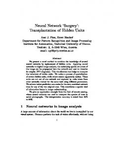
B. M. Wilamowski, N. Cotton, J. Hewlett, 0. Kaynak L Neural Network Trainer with Second Order Learning Algorithms

algorithms for the user to choose from: EBP - traditional Error Back Propagation BMW - a modified Levenberg-Marquardt algorithm for arbitrarily connected neural networks. SA - Self Aware algorithm which is a modification of BMW. It evaluates the progress of the algorithms training and determines if the algorithm is failing to converge. If the algorithm begins to fail the weights are reset and another trial is attempted. In this situation the program displays its progress to the user as dotted red line on the display and begins again. The algorithm continues to attempt to solve the problem until either it is successful or the user cancels the process. ESA - Enhanced Self Aware algorithm, which is also a modification of the BMW algorithm, is used in order to increase chances for convergence. The modification was made to the Jacobian Matrix in order to allow the algorithm to be more successful in solving very difficult problems with deep local minima. It is also aware of its current solving status and will reset when necessary. F- ESA -Another modification of the BMW algorithm where an alternative method for calculating the Jacobian matrix is used. The calculation of Jacobian is unique in the sense that only feed-forward calculations are needed. This approach is then paired with the Enhanced Self-Aware LM algorithm. Evolutionary Gradient - newly developed algorithm which evaluates gradients from randomly generated weight sets and uses the gradient information to generate new populations of weights. This is a hybrid algorithm which combines the use of random populations with an approximated gradient approach. Like standard methods of evolutionary computation, the algorithm is better suited for avoiding local minima when compared to common gradient methods such as EBP. What sets the method apart is the use of an approximated gradient which is calculated with each population. By generating successive populations in the gradient direction, the algorithm is able to converge much faster than other forms of evolutionary computation. This combination of gradient and evolutionary methods essentially offers the best of both worlds. The BMW algorithm was briefly described in [15] and the Evolutionary Gradient algorithm was described in [16]. III. ESA - ENHANCED SELF AWARE ALGORITHM A common problem with many training algorithms is that local minima often cause some weights to get pushed into the saturated portion of the tangent hyperbolic curve (see Fig. 4). In the saturated region, the slope is nearly zero and therefore the derivative is also nearly zero. This is a problem when a particular pattern has a large error while in saturation. In this case when the error is multiplied by the slope the error is lost. This causes the algorithms to frequently get stuck in local minima. By scaling the Jacobian by a constant, this allows the patterns to remain in the linear region longer in order to allow all of the patterns to be correctly classified. The downfall of this scaling is that it makes it more difficult to find

the exact solution when the errors are small. To account for this, the algorithm monitors the errors for each pattern and when the errors for all patterns are small the algorithm no longer scales the Jacobian Matrix. This allows the algorithm to converge to a very small error. Saturation _

/ -11,

Fig.

Linear Region

\X J

4Typical acti

4 ationfunt2i o

Fig. 4 Typical activation function Algorithm

______

_____

Success Rate

Scale Sc

l

orBMW

| 79%

N/A

ESA

94%

2.9

BMW

21%

N/A

ESA

70%

2.5

BMW

0%

N/A

n

ESA

43%

4

CD

BMW

17%

N/A

n

ESA

59%

4

n

LO n

TABLE 1. Comparison of BMW and ESA algorithms

The ESA algorithm was compared with the BMW algorithm. At the beginning of each training session random weights are generated as the starting weights for the calculation. These weights can play a significant role in whether or not the algorithm will converge. This makes it difficult to determine if the algorithm is converging because it is working properly or simply because it had a good set of starting weights. In order to remove this variable, a library of random weight sets was generated for each neural network and saved. Each algorithm was tested for each starting set and its convergence was recorded. Based on success rate of the ESA algorithm, it was better than that of the BMW algorithm on every training set compared. The enhanced in many cases took more iterations but this cost is heavily out weighed by the shear ability to converge with a reasonable success rate. Despite the better success rate, the ESA algorithm's convergence was consistently slower then the BMW algorithm. Therefore, it should be used only for very difficult problems.

129 Authorized licensed use limited to: ULAKBIM UASL - BOGAZICI UNIVERSITESI. Downloaded on February 19, 2009 at 07:49 from IEEE Xplore. Restrictions apply.

INES 2007 c 11th International Conference on Intelligent Engineering Systems

IV. F-BMW - FEED-FORWARD JACOBIAN CALCULATION Calculation of the Jacobian matrix is an essential part of the

Levenberg-Marquardt algorithm. Although using the Jacobian for approximating the Hessian matrix significantly reduces computational complexity, calculating the Jacobian can be rather involved by itself. The method for calculation traditionally used by the Levenberg-Marquardt training algorithm requires both forward and backward calculations. First, feed forward calculations are made to determine the error. The elements of the Jacobian matrix are then obtained by propagating this error back through the network. It is this backwards calculation which is largely responsible for the algorithm's relative complexity. A simpler method is proposed which closely approximates the Jacobian matrix using only feed-forward calculations. A. A short derivation The proposed method requires that the elements of the Jacobian matrix be expressed as a function of the net input for each neuron in a given network. A short derivation is required in order to obtain this relationship. The Levenberg-Marquardt algorithm computes the elements of the Jacobian matrix in the form

J(i, j)=

ae1i

awj

(1)

where e1 is the error for the input pattern xi, and Wj is a specific weight. The first step in the derivation is to find a relation between ao andae . The error associated with a given input pattern is defined as the difference between the desired output and the actual output for a specified set of weights, or (2) ek = od Ok where od is the desired output for the given pattern and ok is the actual output generated using the weight set wk, with k being the number of the current iteration. The change in outputs between iterations k and k -1 is simply (3) o-=ok -°k-I Thus, solving (2) for ok and substituting into (3),

ao= od ek °k-I (4) Finally, substituting k -1 for k in (2) and combining it with (4) yields the desired relationship between ao and ae. aO = -d °k-l ek =

ek

-Iek

-

29 June - 1 July 2007 Budapest, Hungary -

O = f(net)

where f is the activation function of the neuron. For the general case in which the neuron has n inputs including the bias, net =w1 X1 +W2 .X2

+***+Wn Xn

With this in mind (5) can again be rewritten, this time relating it to net.

Doi

awj

=_ aoi

anet

anet

aw,

It is clear from (6) that for any wj,

anet

JX

Thus

J(i, j=

-

Do1 8ni

anet

x

J(i,) = -

aOi

(7)

B. Approximating the Jacobian

The only unknown term in (7) is aoi anet, which corresponds to the gain between the input of the given neuron and the output of the network. This gain can be approximated numerically by slightly incrementing the value of net and then dividing the corresponding change in output by the size of the increment. With this value for aoi I anet, the corresponding element of the Jacobian matrix can be easily approximated using (7). By this method, the entire Jacobian matrix can be obtained using the gains associated with each of the neurons. Because these gains can be computed using only feed-forward calculations, no back-propagation is required. The single drawback to this method is that its accuracy depends entirely on the size of anet . As anet approaches zero, the accuracy of the approximation increases, however the bit precision required to compute each of the elements also increases. This puts a limit on the level of accuracy which can be achieved. C. Results from testing Three separate networks were trained using the proposed method in conjunction with the modified LM algorithm described in section IV. The networks were trained 100 times each using a set of one hundred randomly generated starting weights. Each network was then retrained using the unmodified LM algorithm and standard Jacobian. The same set of initial weights was used for comparison. A comparison of the results is shown in the table below.

> ao =-e The Jacobian can now be expressed in terms of the change in

output rather than error.

(6)

(5)

This relationship is useful since, for a given neuron, the output is a function of the net input, or

130 Authorized licensed use limited to: ULAKBIM UASL - BOGAZICI UNIVERSITESI. Downloaded on February 19, 2009 at 07:49 from IEEE Xplore. Restrictions apply.

B. M. Wilamowski, N. Cotton, J. Hewlett, 0. Kaynak A Neural Network Trainer with Second Order Learning Algorithms

|Success Rate

|AlgorithmAlgorithm | Jacobian

Failure

Rate

>

BMW

Standard

79%

21%

.

ESA

Feed-forward

95%

5%

LO

BMW

Standard

21%

79%

0-

.>

ESA BMW

Feed-forward Standard

59% 0%

41% 100%

0-

ESA

Feed-forward

When the BMW algorithm was applied for the same set of patterns and the same starting weights, both the success rate and convergence time were improved drastically. Results are shown in Figs. 7 and 8. 10 0

37%

63%

TABLE 2. Comparison of BMW and ESA algorithms using feedforward computation of Jacobian

Although the feed-forward method for calculating the Jacobian is only an approximation, when paired with the ESA algorithm, it has a better success rate than BMW algorithm. However for BMW it converges much faster if it converges at all. V. EXPERIMENTAL RESULTS

10 10

-2

10

-3

10

-4

10

-5L

20

30

25

3b

Fig. 7. Results of BMW algorithm using a traditionally connected network for a parity-3 problem. 10 10

Algorithms implemented in the Neural Network Trainer (NNT) were compared on several difficult problems starting with parity problems. Figures 5 and 6 show results for the parity 3 problem using EBP. The figures were generated using layered and fully connected networks respectively. One may notice that for a fully connected network EBP converges faster and has a better success rate.

lb 1

1

1 00

0

10 10

-2

10 -3 10 10

-4 -5

2

4

6

8

10

12

16

14

18

20

10

Fig. 8 Results of BMW algorithm using a fully connected network for a parity-3 problem.

E 64

22-

-2

41

0

100

200

300

400 500 600 Number of Itereations

700

800

900

1000

Fig. 5 Results of EBP algorithm using a traditionally connected network for a parity-3 problem. 10 ' 8l

vA

E 6 0)

4-

°

2

L

lo

'

o

US

1

15

2

25

3

35

4

45

5 x

_

104

Fig. 9. Results of EBP algorithm a fully connected network for a

parity-5 problem. 4

0

100

200

300

400 500 600 Number of Itereations

700

800

900

1000

Fig. 6. Results of EBP algorithm using a fully connected network for a parity-3 problem.

For a more complex problem like parity 5, the EBP algorithm failed in all tried cases despite 50,000 iterations (Fig. 9). When ESA algorithm was used, it reached the solution in 100% of the cases with an average of about 100 iterations. The results are shown in Fig. 10. The ESA algorithm was also successful in 48% of cases for the parity-7 problem (Fig. 11).

131 Authorized licensed use limited to: ULAKBIM UASL - BOGAZICI UNIVERSITESI. Downloaded on February 19, 2009 at 07:49 from IEEE Xplore. Restrictions apply.

INES 2007

11th International Conference on Intelligent Engineering Systems

-

25 Runs for Parity 5

10 10

10

10X 10 10 1

10

l, ''' ' 'l

02

0

20

40

', 11'',

60 80 Iterations

F

100

120

140

10. Results of ESA algorithm a fully connected network for a Fig. ol10 ll' parity-S problem. Runs for Parity 7 ~~~~~~~25

3

10

10 102

10-3

10

0

100

200

300

400 Iterations

500

600

700

800

Fig. 11. Results of ESA algorithm a fully connected network for a parity-7 problem.

VI. CONCLUSION The Neural Network Trainer with Second Order Learning Algorithms was described. The software was developed in the MIATLAB environment and has a user friendly interface. It is capable of training feed-forward neural networks with arbitrary architectures. The network topology is entered in a manner similar to the SPICE program. Several second order algorithms are implemented which are able to more efficiently train neural networks. It was also shown that fully connected neural network architectures are more efficient than commonly used layer by layer architectures. The NNT software is available as either a stand alone executable or as a p-file which will run in MIATLAB. Both versions are available for download at

http: /www.eng.auburn.edu/-wilambm/NNT.zip. VII. REFERENCES

-

29 June - 1 July 2007 Budapest, Hungary -

[2] Da Silva, L.E.B.; Bose, B.K.; Pinto, J.O.P.; "Recurrent-neuralnetwork-based implementation of a programmable cascaded low-pass filter used in stator flux synthesis of vector-controlled induction motor drive," IEEE Transactions on Industrial Electronics Volume 46, Issue 3, June 1999 pp. 662 - 665 [3] Bimal K. Bose, "Neural Network Applications in Power Electronics and Motor Drives An Introduction and Perspective," Trans. on Industrial Electronics, vol. 54, no. 1, pp. 14-33, Feb. 2007. [4] Baburaj Karanayil, Muhammed Fazlur Rahman, Colin Grantham, "Online Stator and Rotor Resistance Estimation Scheme Using Artificial Neural Networks for Vector Controlled Speed Sensorless Induction Motor Drive," Trans. on Industrial Electronics, vol. 54, no. 1, pp. 167-176, Feb. 2007. [5] Ahmed Rubaai, Marcel J. Castro-Sitiriche, Moses Garuba, III Legand Burge, "Implementation of Artificial Neural NetworkBased Tracking Controller for High-Performance Stepper Motor Drives," Trans. on Industrial Electronics, vol. 54, no. 1, pp. 218-227, Feb. 2007. [6] Seul Jung, Sung su Kim, "Hardware Implementation of a RealTime Neural Network Controller With a DSP and an FPGA for Nonlinear Systems," Trans. on Industrial Electronics, vol. 54, no. 1, pp. 265-271, Feb. 2007 [7] Wilamowski, B.M, Neural Networks and Fuzzy Systems, chapter 32 in Mechatronics Handbook edited by Robert R. Bishop, CRC Press, pp. 33-1 to 32-26, 2002. [8] Rumelhart, D. E., Hinton, G. E. and Wiliams, R. J, "Learning representations by back-propagating errors", Nature, vol. 323, pp. 533-536, 1986. [9] B. M. Wilamowski and D. Hunter, "Solving Parity-n Problems with Feedforward Neural Network," Proc. of the IJCNN'03 International Joint Conference on Neural Networks, pp. 25462551, Portland, Oregon, July 20-23, 2003. [10] SNNS (Stuttgart Neural Network Simulator) - http://www-

ra.informatik.uni-tuebingen.de/SNNS/ [11] Scott E. Fahlman. Faster-learning variations on backpropagation: An empirical study. In T. J. Sejnowski G. E. Hinton and D. S. Touretzky, editors, 1988 Connectionist Models Summer School, San Mateo, CA, 1988. Morgan Kaufmann. [12] M. Riedmiller and H Braun. A direct adaptive method for faster backpropagation learning: The RPROP algorithm. In Proceedings of the IEEE International Conference on Neural Networks 1993 (ICNN93), 1993. [13] S.E Fahlman, .and C. Lebiere, "The cascade- correlation learning architecture" in D. S.Touretzky, Ed. Advances in Neural Information Processing Systems 2, Morgan Kaufmann, San Mateo, Calif, (1990), 524-532. [14] M.T. Hagan. M.B. Menhaj. "Training feedforward networks with the Marquardt algorithm." IEEE Trans. on Neural Networks 1994; NN-5:989-993. [15] B. Wilamowski, N. Cotton, 0. Kaynak, and G. Dundar, "Method of computing gradient vector and Jacobian matrix in arbitrarily connected neural networks" ISIE 07 IEEE International Symposium on Industrial Electronics, Vigo, Spain, June 4-7, 2007. [16] J. Hewlett, B. Wilamowski, and G. Dundar "Merge of Evolutionary Computations with Gradient Based Method for Optimization Problems" ISIE 07 EEE International Symposium on Industrial Electronics, Vigo, Spain, June 4-7, 2007.

[1] Embrechts, M.J.; Benedek, S.; "Hybrid identification of nuclear power plant transients with artificial neural networks," IEEE Transactions on Industrial Electronics Volume 51, Issue 3, June 2004 pp. 686 - 693

132 Authorized licensed use limited to: ULAKBIM UASL - BOGAZICI UNIVERSITESI. Downloaded on February 19, 2009 at 07:49 from IEEE Xplore. Restrictions apply.