NEURAL NETWORKS FOR ADMISSION CONTROL IN AN ATM NETWORK Ernst Nordström, Olle Gällmo and Lars Asplund Department of Computer Systems Box 325, S–751 05 Uppsala Uppsala University, SWEDEN and Mats Gustafsson and Bo Eriksson Circuits and Systems Group Department of Technology Box 534, S–751 21 Uppsala Uppsala University, SWEDEN mail:
[email protected] ABSTRACT This paper presents an artificial neural network (ANN) approach to link admission control in ATM communication networks. Three different ANN models for implementation of link quality of service formulas, based on a heterogeneous fluid–flow queueing model, are presented. The first model uses predefined peak rate parameters, the second model is based on a state interpretation of aggregated link traffic, and the third model employs a form of statistical pre–processing of the traffic parameters.It is argued that the ANN must implement a function which is invariant to every permutation of the traffic descriptor arguments. This constraint is met by the third ANN model and the experiments presented also suggests that the pre–processing performed is benificial for generalization situations.
1 INTRODUCTION The Asynchronous Transfer Mode (ATM) is intended to be the basis for a future Broadband Integrated Services Digital Network (B–ISDN). ATM is a packet–oriented switching and multiplexing technique designed to meet different bandwidth and Quality Of Service (QOS) demands of B–ISDN services [1]. Today, much effort is put in research & development of ATM technology, especially within the area of congestion control. Call admission control is a key part in preventive congestion control. Different analytical approaches have been proposed to develop an effective admission control criterion. Although accurate performance models of the link traffic exist, e.g. the fluid flow queueing model for heterogeneous on/off traffic, they are too complex to be used in a real ATM network. Instead, approximations are done to meet ATM response time constraints [2–4]. In this paper another approach is proposed. Instead of simplifying the performance model at the price of inaccurate results, artificial neural networks (ANNs) are used to reproduce the behaviour of an accurate performance model. An important remark about the performance models is that they only consider the declared traffic profiles as opposed to [5] where neural networks are used for call admission control based on actual traffic. In [6] the latter method is extended to solve integrated admission and link capacity control problems.
2. ATM NETWORK 2.1 ATM Switching An ATM network combines the advantages of packet and circuit mode by switching fixed sized labeled ”cells” through virtual circuits. The ATM access nodes multiplex user cells onto high capacity links for transmission to inner ATM nodes (switches). The ATM switches perform cell routing and multiplexing according to the cell labels. Several virtual circuits usually share a single transmission link to improve network utilization. The ’by– need’ allocation of bandwidth means that the network behaves as a system employing statistical multiplexing. 2.2 Congestion Control Conflicts may arise when cells belonging to different virtual circuits simultaneously are switched to the same outlink. This holds even if the outlets are equipped with buffers to queue competing cells, since the buffers may be momentarily saturated. Also, the queues introduce cell delays and cell delay variations, which might be critical for some services. Consequently a virtual circuit’s QOS, e.g. cell loss ratio and cell delay, can only be guaranteed in a probabilistic sense. In order to maintain the negotiated QOS it is necessary to avoid congestion in the network. An efficient load control mechanism is thus of prime importance. The approach taken in this paper is that of preventive load control, i.e. connection requests which might lead to congestion are not accepted, and the data flow entering the network is supervised by a flow enforcement function. 2.2.1 Admission Control The virtual circuit/connection set–up phase contains two parts. First the route through the network is determined. Then a decision is made on each link whether or not to accept the requested connection. The second part uses an algorithm called Admission Control (AC). The purpose of AC is to map the parameters describing the aggregate connections on the link and the parameters of the new connection into a QOS measure, and compare it with the desired QOS. If the desired QOS can be fulfilled the connection is accepted. In order to make correct decisions the AC must use an adequate link performance model. Analytical models of different complexity have been developed [2]. All models are based on queueing theory and use different degrees of approximation. The most accurate approximation proposed in [2] is the fluid flow queueing model for heterogeneous on/off traffic. But, as the connection set–up time is constrained, this rather complex model cannot be used and further approximations must be made. Although such approximations are given, e.g. binomial or Pascal multi server approximations, these performance models often overestimate the cell loss ratio. 2.3 Traffic Modelling 2.3.1 Source Models The ATM network is supposed to carry many different traffic types, including Continuous Bit Rate (CBR) and Variable Bit Rate (VBR) services. A versatile traffic source model admitting analytical QOS calculations is therefore needed. The on/off source model meets these requirements. In this model a source is either in an on–state, producing cells at a constant generation rate f, or in a silent off–state. The duration of the on–state (off–state) is expected to be exponentially distributed with mean ton (toff).
2.3.2 Control Time Scales ATM congestion control is considered to be performed in different time scales. These are the cell level, the burst level and the connection level. The connection level is the uppermost level, and considers variations in the number of established connections. The burst level considers the variation in cell arrival rate due to the sources’ transitions between on and off– states. At the cell level individual cells are considered and queueing theory is used to obtain performance data. 2.4 Quality of Service (QOS) Since B–ISDN will support a wide range of services the ATM network will face many different QOS demands. For example, low cell delay is more important for voice and video traffic than for high–speed data. On the other hand, high–speed data may be very sensitive to cell loss, while voice traffic can accept a moderate cell loss ratio. In this paper we only consider the cell loss ratio. In order to meet the different demands of QOS the cell loss ratio must be kept at the same order of magnitude as the bit–error–rate which implies a restrictive cell loss ratio of 10 –9. Thus, connection requests which lead to higher cell loss ratios than 10–9 are rejected. 3 A LINK PERFORMANCE MODEL If the buffer size is sufficiently large the discrete cell flow can be approximated with a continuous cell flow leading to a fluid flow queueing model. The buffer is modelled as a fluid reservoir with a hole in the bottom, where arrival cells are flowing into the buffer and departure cells are flowing out of the buffer. A fluid flow model for a finite number of heterogeneous on/off sources is formulated in [3]. Performance formulas such as the overall cell loss ratio are given in the finite buffer case. In this model, the heterogeneous sources are partitioned into c classes, where sources in a given class are statistically identical. Class j, j = 1,...c, are described by the number of sources: Nj the sources’ constant cell generation rate in the on–state: f j the sources’ average duration of the on(off) state: ton(j) (toff(j)) Sometimes the mean cell generation rate, mj, is used as a third parameter, eliminating one of the source parameters above. This parameter is simply the peak generation rate f j multiplied with the fraction of time the source is in the on state: t on(j) mj + fj t on(j) ) t off(j)
The collection of heterogeneous sources is described by the source number vector: N = (N1,..., Nc ) the peak rate vector: f = (f1,..., fc) the average on (off) duration vector: ton = (ton(1),...,t on(c)) (toff = (toff(1),...,t off(c))) One of the source parameter vectors can be replaced with the mean rate vector, m = (m1,..., mc). The maximum output rate from the buffer, denoted fout, and the buffer capacity, denoted B, are also used in the derivations. The cell loss ratio can be shown to be a function of the parameters above, i.e. Ploss = Ploss (N, f, ton, toff , fout, B). A vector k=(k1,k2,...,k c), 0 ≤ kj≤ Nj, that describes a specific combination of on–sources is also used in the derivations, which reference [3] presents in detail. To summarize, the calculation of cell loss is performed in three steps. First, the equilibrium buffer distribution, Fk(x), for different combinations, k, of on–sources is determined. This distribution describes the time independent probability that the sources are in state k and that the buffer content does not exceed x. Then, the probability that the sources are in state k and that the buffer content does exceed x, uk(x), is obtained from the equation qk = Fk(x) + uk(x), where qk is the overall probability that the sources are in state k. qk may be derived from the fact that the number of on (off) sources in a given class are binomial distributed. The equation holds since the buffer content is either ≤ x or > x. Finally, the fraction of lost information to offered information, i.e. the cell loss ratio, is calculated as:
P loss +
ȍ{ k | k @f uf
k @ f * f out) u k(B) N @m
out }
(
where the dot denotes scalar vector multiplication.
4 A NEURAL NETWORK APPROACH 4.1 Introduction The speed – accuracy dilemma that faces the AC algorithm suggests an artificial neural network (ANN) approach. Using parallel distributed processing [9–10], fast admission decisions are possible without approximations of performance models. The idea is to use an ANN to replicate the behaviour of a sufficiently accurate performance model, in our case the heterogeneous fluid flow model. Since the admission control is based on an accurate performance model, a higher number of accepted connections is possible, resulting in a more economical ATM network utilization. 4.2 ANN Modelling 4.2.1 Symmetry Constraint Consider a situation where n–1 connections statistically share an output link and that there is a request for an n’th connection. Let xk = (fk, mk, ton(k)), denote a parameter vector representing connection k (k=1, ..., n). The parameters f k, mk and ton(k) denotes the peak rate, mean rate and on duration as before. The aggregated connection on the link, with connection n accepted, is described by a individual parameter vector Xn = (x1, ..., xn). Thus, the ANN should perform the mappings X n ³ Ploss ³ {accept, reject}, where the final mapping is based on a comparison with the restrictive cell loss ratio 10 –9. Now, assume that the n connections can be partitioned into c different classes with statistically identical sources. Let Nj,k denote the number of sources in class j (j=1, ..., c) after connection k is accepted. Similarly, let yj,k = (Nj,k, fj, mj, ton(j)) denote a vector representing source class j after connection k is accepted. With this notation, the aggregated connection is described by a class parameter vector Yn = ( y1,n, ..., yc,n), and the ANN task becomes Y n ³ Ploss ³ {accept, reject} . A first attempt would be to use a multi layer perceptron (MLP) with 3n input nodes in the first case, and 4c input nodes in the second case. This approach suffers from the fact that the network output should be the same for every permutation of the elements of Xn (Yn). In other words the MLP must learn n! (c!) different versions of Xn (Yn) which soon gets unmanageable. This constraint, which we call the symmetry constraint, has been identified as a key issue in our ANN approach. 4.2.2 Model A: Predefined Peak Rates The first ANN model is based on a finite number of predefined peak rates. If we use fixed peak rates the class parameter vector can be reduced to z j,k = (Nj,k, mj, ton(j)). Denoting the resulting aggregated vector by Zn = ( z1,n, ..., zc,n), the ANN’s task becomes Z n ³ P loss ³ {accept, reject} .
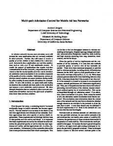
Now, since the peak rates are fixed, we can use an MLP with 3c inlayer nodes and associate three nodes to each class. Thus, the problem of symmetry is avoided by using class–dedicated input node triplets. Since it seems difficult to divide the B–ISDN services into a finite number of fixed traffic classes, i.e. classes with fixed peak rates, mean rates and on durations, a versatile ANN model must have some generalization properties. The ANN model described above can be used to generalize in the parameters N j, mj and ton(j) but not in the parameter fj. The peak rate is chosen as the parameter with predefined values since the services’ mean rates and on durations seem difficult to predict. Also, if we want to change the set of predefined peak rates, e.g. because a service with unknown peak rate is to be carried by the ATM network, it is always possible to re–train the MLP off–line, and then use the extended MLP in the admission control procedure. 4.2.3 Model B: A State Interpretation of Aggregated Traffic In the second ANN model a state vector Sk is used to describe the k connections on the link. The state vector should, besides from being an accurate description of the traffic situation, also contain information about the cell loss ratio. As a first approximation of the state vector we have chosen the tail buffer distribution function, u(x), which express the probability that an arriving cell finds a buffer level that is higher than x: u(x) = Σk uk(x). uk(x) is, as described in section 3, the probability that the sources are in state k and that the buffer content exceed x. The state vector is obtained by evaluating u(x) for different buffer levels. Figure 1 shows three example distributions.
Figure 1. Buffer distribution functions for three different traffic situations. Note that the probability to find the buffer occupied to a certain level increases with the number of connections (N1 ).
Let Sn–1 denote a state vector describing the n–1 connections already sharing the link and let xn describe the new connection. The ANN under consideration maps the state vector Sn–1 and the parameter vector xn to a new state Sn: (S n*1, x n) ³ S n ³ P loss ³ {accept, reject} . Note that instead of the symmetry constraint stated above, we face the constraint that the state Sn must be independent of the order of the connection requests. Since the n connection requests can appear in any order, n! different sequences are possible. For example, consider the connection requests xa and xb. The sequence constraint means that the ANN output for (Sa, xb) and (Sb, xa) must be the same. 4.2.4 Model C: Higher–Order Inputs In the third ANN model the symmetry constraint is removed by using an MLP with higher–order inputs which are determined from symmetry considerations. The symmetry constraint means that the ANN must implement a function, g=g(x1,...,xn), which is invariant to every permutation of the arguments xk (k=1, ..., n). That is, g’s dependency of the parameters fk, mk and ton(k) of xk must be the same for every k (property 1). Similarly, g’s dependency of the parameter variations and covariations must be the same for every k (property 2). This must also hold for the parameter covariations between different k (property 3). To state this more formally we introduce the second order Taylor expansion of g at the origin: g(x1, ..., xn) = g(0) + Σi (rxi)T g(0) xi + 1/2 Σi Σj xi (rxi)T rxj g(0) xjT, where, using the notation xk=(αk, βk, γk), rxi = (∂/∂αi , ∂/∂βi , ∂/∂γi) and
(rxi) Τ rxj
ȡ∂ń∂αi∂α j ∂ń∂α i∂βj ∂ń∂β ∂α ∂ń∂β ∂β +ȧ ȧ∂ń∂γ i∂α j ∂ń∂γ i∂β j i j Ȣ i j
∂ń∂αi∂γjȣ ∂ń∂β i∂γ jȧ ∂ń∂γi∂γj
ȧ Ȥ.
The symmetry constraint can now be stated as rxi g(0) = D, (rxi)T rxi g(0) = H (rxi)T rxj g(0) = G
i,j = 1, ...., n, and j ≠ i.
Notice that D is a constant vector corresponding to property 1. H and G are constant matrices corresponding to property 2 and 3 respectively. Substituting the constraint expressions and xk=(αk, βk, γk) into the Taylor expansion yields g(x1, ..., xn) = g(0) + D Σi xi +1/2 [ Σi xi H xi T + Σi Σj ≠ i xi G xjT ] = = g(0) + d1Σi αi + d2Σi βi + d3Σiγi + 1/2[ h11Σi(αi)2 + h22Σi(βi)2 + h33Σi(γi)2 + h12Σiαiβi + h13Σiαiγi + h23Σiβiγi + g11ΣiΣj ≠ i αiα j + g22ΣiΣj ≠ i βiβj + g33ΣiΣj ≠ i γiγj + g12ΣiΣj ≠ i αiβj + g13ΣiΣj ≠ i αiγj + g23ΣiΣj ≠ i βiγj ].
di denotes an element of vector D, hij and gij denotes elements of the matrices H and G. In the last equality the (Hessian) properties hij = hji and gij = gji have been used. The number of summations can be reduced by noticing g(x1, ..., xn) = g(0) + d1Σi αi + d2Σi βi + d3Σiγi + 1/2[ (h11 – g11)Σi(αi)2 + (h22 – g22)Σi(βi)2 + (h33 – g33)Σi(γi)2 + (h12 – g12)Σiαiβi + (h13 – g13)Σiαiγi + (h23 – g23)Σiβiγi + g11(Σiαi)2 + g22(Σiβi)2 + g33(Σiγi)2 + g12(Σiαi)(Σiβi) + g13(Σiαi)(Σiγi) + g23(Σiβi)(Σiγi)]. The idea is to use the sums and product of sums (henceforth called components) described above as higher order inputs to an MLP. That is, instead of training the MLP to recognize every permutation of the parameter vectors, the symmetry problem is solved by pre–processing of parameter data. Let Tj,n denote component number j (j=1,...,15) when n connections are accepted, i.e. T1,n = Σαi, T2,n = Σβi, ..., T15,n = (Σβi)(Σγi), and let Tn denote the aggregated vector Tn = (T1,n,T2,n, ...,T15,n). Using this notation the ANN task becomes T n ³ P loss ³ {accept, reject} . An analysis of the 15 components shows that these may be found in the expressions for sample mean, variance and covariance. The components of type Σαi is simply the nominator in the expression for the arithmetic mean of αi ma +
ai n
The components of type Σ(αi)2 and (Σαi)2 may be found in the sample variance expression for αi since va +
1 [ n*1
ȍ(a )
2
i
*
1
ȍa) ] .
n(
2
i
Similarly, the components of type Σαiβi and (Σαi)(Σβi) may be found in the sample covariance expression for αi and βi, c ab +
1 [ n*1
ȍab i
i
*
1
n(
ȍ a )(ȍ b )] . i
i
Note that if we use the means (mα, mβ, mγ), variances (vα, vβ, vγ), covariances (cαβ, cαγ, cβγ) and the number of connections n as inputs we a can not guarantee equal classification quality since this data contains slightly less information than the original components. That is, the statistical data only permits 10 degrees of freedom compared to 15 for the Taylor components. 4.3 Experiments 4.3.1 Parameter Constraints The experiments described below are based on cell loss calculations using the heterogeneous fluid flow model. A program written by S. Jacobsen [2–3] is used for generation of cell loss data. In this program, only three source classes can be used simultaneously, and the
number of sources in these classes is restricted by (N 1+1)(N2+1)(N3+1) ≤ 750 due to memory limitations. Since the performance model only considers load situations where the mean offered traffic is less than the output link capacity the number of sources and mean rates are restricted by N1m1 + N2m2 + N3m3 < fout, where of course mj ≤ fj. The fact that no cell loss is possible when the sum of the peak rates is less than the output link capacity, i.e. N1f1+ N2f2+ N3f3 < fout, has been used to reduce the number of program runs. Furthermore, the peak rates fj should be less than 10% of the output link capacity in order to gain from statistical multiplexing [7–8]. 4.3.2 Generation of Sample Sets Consider the crucial task of selecting parameter combinations for cell loss evaluation. The goal is to determine a parameter distribution which enables correct ANN classifications. In this context it may be pointed out that the parameters fj, mj and ton(j) have decreasing importance, i.e. the parameter density in the peak rate dimension should be higher than in the mean rate dimension etc. The performed ANN experiments are based on sample sets containing pairs of class parameter vectors Yk = ( y1,k, y 2,k, y3,k) and cell loss values Ploss,k. The vectors Yk contain unique N1, N2 and N3 combinations for fixed choices of fj, mj and ton(j) (j=1,2,3). Seven sample sets {(Yk, Ploss,k)} with different source class characteristics have been generated, see table 1. The peak rate parameters are the same in all sets while the mean rate and on duration parameters differ. The number of connections have been varied in steps of three for class 1 and 2 and in steps of two for class 3. Future experiments will consider the relative importance of the parameters more extensively, i.e. more samples with varying peak rates will be generated. In the cell loss calculations, a buffer capacity B of 100 cells is used. This choice gives sufficient ATM network efficiency according to [2]. The output link capacity fout is chosen to 135 Mbit/s (instead of 155 Mbit/s). This is motivated by the reduced transfer efficiency induced by cell overhead and frame synchronization cells [2].
Set#
#Samples f1
m1
ton(1)
f2
m2
ton(2)
f3
m3
ton(3)
1 2
796 553
2 2
1 1
25 12
6 6
2 2
8 8
12 12
3 3
4 4
3
497
2
1
25
6
2
4
12
3
4
4
362
2
1
25
6
2
8
12
6
4
5
267
2
1
25
6
2
8
12
8
4
6
193
2
1
25
6
4
8
12
8
4
7
286
2
1
25
6
4
8
12
6
8
Table 1. Traffic profiles for generated sample sets. The peak rate fj and the mean rate mj are given in Mbit/s and the on duration ton(j) in msec.
4.3.3 Model A The model A which is based on a set of predefined peak rates has been examined for 6 different combinations of training and test sets, see table 2. Normalized versions of the sample sets were used. The input vector elements were normalized to the interval [0,1] and the cell loss values were logarithmized and mapped to the interval [–1,1]. Test no.
Learned Test Sets Set
1
1
2
2
1
3
3
1,5
4
4
1,4
5
5
1,4
7
6
1,4,6
7
Table 2. Composition of training and test sets. Two MLPs with 2 respectively 5 hidden nodes were used in the experiments which table 3 summarizes. The table shows that the MLP with 5 hidden nodes performs better than the MLP with 2 hidden nodes when the generalization task is more difficult, e.g. for test no. 4 and 5. Both MLPs have very good results for test no. 3, which is natural since the test classifications only involves interpolations. Test no.
2 Hidden Nodes % correct (s) Train Test
5 Hidden Nodes % correct (s) Train Test
1
94.8 (2.6)
93.7 (3.7)
96.5 (2.3)
93.9 (3.5)
2
96.5 (2.6)
91.8 (5.4)
97.1 (1.3)
92.6 (3.1)
3
95.2 (1.8)
96.8 (1.6)
94.6 (2.0)
95.2 (2.4)
4
95.0 (3.1)
90.8 (6.4)
95.6 (1.9)
95.4 (1.9)
5
96.6 (1.5)
78.3 (7.6)
96.6 (2.1)
85.1 (7.0)
6
94.4 (3.0)
84.8 (7.5)
96.2 (2.1)
84.3 (8.0)
Table 3. Experimental results (% correctly classified patters, 10 times average) after 100 epochs of training for model A. The figures within parentheses are standard devi– ations (s). 4.3.4 Model B Only a small amount of experiments have been performed with the model B based on a state interpretation of aggregated traffic. This is because the choice of the buffer distribution function as the state vector was found to give numerical problems. Since the model uses successive mappings (S k*1, x k) ³ S k a state vector must be accurate even for light load situations. Unfortunately the buffer distribution function is poor at describing very light load situations
since the probability to find cells in the buffer is very low. Furthermore, even if a very high accuracy is used in the generation of buffer distribution data, a neural network will have difficulties to implement such an accuracy. This is an important remark since one false state vector is sufficient to reduce the classification quality. The same program that was used for the cell loss calculations has been used in the generation of buffer distribution data. A state vector was estimated by evaluating this function at 9 different buffer levels. These samples were chosen to best represent the function, i.e. more samples were taken for low buffer levels. The logarithm of the values were taken to concentrate the sample distribution and the training set was normalized, producing state vector elements in the interval [0,1]. Then, an MLP with 5 hidden nodes were trained to associate (Sk–1, xk) combinations to state vectors Sk. The experiments confirmed the numerical difficulties described above. Furthermore, the wide scattering of buffer distribution data resulted in poor training performance for some examples. 4.3.5 Model C The model C which uses pre–processing based on symmetry considerations has been examined using the same data as for model A. Again, two MLPs with 2 respectively 5 hidden nodes were used in the experiments, which table 4 summarizes. A comparison of the results of model A & C shows that model C has similar properties for the first three tests. For the last two tests model C performs better than model A, the result is about 10% higher for model C. As Table 1 shows, the traffic parameters for these tests are more difficult, i.e. the model A network has to extrapolate for some of the test samples. Thus, it seems that the linearisation performed by the pre–processing is beneficial for extrapolation situations. Test no.
2 Hidden Nodes % correct (s) Train Test
5 Hidden Nodes % correct (s) Train Test
1
97.1 (1.4)
88.7 (2.4)
97.7 (1.4)
93.5 (1.7)
2
96.3 (1.6)
90.6 (3.5)
97.9 (1.4)
92.7 (1.8)
3
96.1 (2.3)
96.9 (2.2)
96.4 (2.5)
97.2 (2.1)
4
96.3 (1.4)
95.5 (1.4)
97.6 (1.8)
96.2 (1.6)
5
97.3 (1.7)
96.4 (0.5)
97.6 (0.8)
96.8 (0.4)
6
97.0 (1.4)
97.0 (1.0)
97.2 (1.4)
97.4 (0.8)
Table 4. Experimental results (% correctly classified patters, 10 times average) after 100 epochs of training for model C. The figures within parentheses are standard deviations (s). 5 CONCLUSION This paper has presented different artificial neural networks models for admission control in ATM networks. It is pointed out that the admission criteria should be based on an accurate link performance model since this allows higher utilization of the ATM network. Therefore a neural network is proposed to reproduce accurate cell loss calculations performed by the heterogeneous fluid flow model. Three different ANN models are exploited; the first model uses predefined peak rate parameters, the second model is based on a state interpretation of aggregated link traffic, and the third model employs a form of statistical pre–processing of the traffic parameters.
ACKKOWLEDEMENT The authors would like to thank Anders Törnqvist and Daniel Fagerström for their contributions in discussions of our work. We also acknowledge ELLEMTEL Telecommunications Laboratories for financially supporting this project called ”Hardware Implementation of Neural Networks for Applications in the Telecom Area”. REFERENCES 1
Händel R. & Huber M.N, Integrated Broadband Networks: An Introduction to ATM–based Networks, Addison–Wesley, 1991.
2
Jacobsen S., Moth K. & Dittmann L., Load control in ATM networks, Proceedings of ISS 90, Stockholm, Sweden, Vol. 5, pp 131–138, May 1990.
3
Jacobsen S., Dittman L. & Moth K., A fluid flow queueing model for heterogeneous on/off traffic, Proceedings 8th Nordic Teletraffic Seminar, Otnas, Finland, Aug 1989.
4
Andersson H. & Andersson H., On analytical models for multiplexing in ATM networks, Lund Institute of Technology, Department of Communications Systems, Nov 1991.
5
Takahashi T. & Hiramatsu A., Integrated ATM traffic control by distributed neural networks, ISS 90, Stockholm, Sweden, Vol. 3, pp 59–65, May 1990.
6
Hiramatsu A., Integration of ATM call admission control and link capacity control by distributed neural networks, IEEE Journal on Selected Areas in Communications, Vol 9, no 7, pp 1131–1138, Sep 1991.
7
Habib I. & Saadawi T., Controlling flow and avoiding congestion in broadband networks, IEEE Communications Magazine, Vol 29, no. 10, pp 46–53, Oct 1991.
8
Roberts J., Variable–bit–rate traffic control in B–ISDN, IEEE Communications Magazine, Vol 29, no. 9, pp 50–56, Sep 1991.
9
Kosko B., Neural Networks and Fuzzy Systems, Prentice Hall, 1992.
10
Rumelhart D., Hinton G. & Williams R., Learning internal representations by error propagation, Parallel Distributed Processing, MIT Press, Vol 1, pp 318–362, 1986.