Theorem, the full conditional posterior distributions ... the kernel estimator, based on the Rao-Blackwell theorem, given by Gelfand and Smith (1991). End of 1th ...
Non Linear State Space Models and Gibbs Sampling applied to Fisheries Stock Assessment
MEMPES, Department of General Economy and Statistics, University of Huelva (Spain)
Isabel Serrano Czaia, Mª Dolores González Galán, Juan José García del Hoyo Description of the Fishery
F ( S t-1 )
S t-1
St = Xt-Pt
Xt Close season
St
Xt
Fishing season Xt '
Beverton-Holt
The way to capture this species is with trawlers, surrounding the fish soal and enclose them in both sides and underneath.
Mackerel (Scomber Japonicus)
Spawning stock
Recruitment
Pt
Capture
Et
Effort
% β St&&1 1%
Xt ' α St&&1 e
(
)
)
1 w t ≈ N 0 , hw = 2 σw 1 v t ≈ N 0 , hv = 2 σv
2 6. 5
1 50 0
26 2 5. 5
1 00 0
Starting vector:
1 97 8
1 98 5
LX00, LX10, ..., LXT0 , "00, "10, $0 , q0, hv0 , hw0
St = X t − Pt
End of 1th iteration
LX01, LX11, ..., LXT1 , "01, "11, $1 , q1, hv1 ,hw1 Repeating the process
Main characteristics of the marginal distributions for the BevertonHolt model parameters K α0 α1 q hv hw LX 0 LX T
Mean 38024,17 5,416 -0,195 0,0000714 403,200 6,259 9,925 9,654
Median 38056,72 5,430 -0,194 0,0000728 394,253 6,249 9,914 9,626
St. Dev. 287,365 0,0705 0,002 0,00000699 162,948 0,517 0,084 0,128
Skewness 0,250 -0,806 -0,528 -2,745 0,236 1,094 3,185 4,147
Jarque -Bera 1374,003 154,626 59,0139 6714,268 15,743 2225,725 14526, 4 25875,5
Probability 0 0 0 0 0,000381 0 0 0
From the data of the tables, the histograms and the estimate densities for these variables, it is followed that all the distributions are bell-shaped, unimodals and in general, slightly skewed. Both models present good results reducing the uncertainty assigned initially.
96 19 99
19
87
93
19
84
90
19
81
78
19
75
19
19
1 w t ≈ N 0 , hw = 2 σw 1 v t ≈ N 0 , hv = 2 σv
Ke r St −1 K + (e r − 1)St −1
t
Initial values of the Beverton-Holt model (S.S.M.(2)) A generalisation of the Schaefer approach, depending on the expected “captures per unit of effort” or CPUE (Ut) of the fishing season in year t, has been used. In this case, we have adapted the equation to the model adding the environmental factor
St ) = α 0 + α1Tt −2 − β St −1 − qEt St −1
Ut +1 − Ut −1 r U − qEt =r− qk t 2Ut
−q E Pe t = wt 1 − e −q E 0
t
0
r = α 0 + α1Tt −2 144444244444 3
t
Assigning an initial value to the parameter q, we obtain a value for wt that will replace St in the Ricker equation, then the coefficients α0, α1, β and q are estimated applying the linear least square approximation. Repeating this process using now the new estimation of q, it will be stopped when the difference between an initial value and the outcome estimation is minimum.
⇓
Ut +1 − Ut −1 α α = α 0 + α1Tt −2 − 0 Ut − 1 Tt −2Ut − qEt 2Ut qk qk (Ut +1 - Ut −1) / 2 Ut = 5.32− 0.19 Tt −2 − 0.001Ut + 7.14E − 5 Tt −2Ut − 7.41E − 5 Et (3.36)
(0.12)
(0.002)
R 2 = 0.53
(3.4E-5)
DW=172 .
(8.15E-5)
F=4 .7
LX02, LX12, ..., LXT2 , "02, "12, $2 , q2, hv2 ,hw2
Results
Probability 0,0749 0,0759 0 0 0,00094 0 0 0
St ⇒ X t = −qE e )
⇒ St ≈
(Geman and Geman, 1984)
Jarque-Bera 5,183 5,156 248,183 2878,612 13,936 524,003 1524,805 10695,91
1 t −2
t
⇓ (Ric ker Equation )
(LX0i, ... ...,, LXTi , "0i, "1i, $i , qi, hvi ,hwi ) - f(LX .., LXT , "0, "1, $ , q, hv, hw) f(LX0 ...,
Skewness -0,167 -0,157 -0,840 -2,078 0,288 -1,470 -1,003 3,075
DW=2.23
Prior Distributions
Generate hw1 from f(hw / LX01, LX11, ..., LXT1 , "01, "11, $1 , q1, hv1) New starting vector
1 t−2
0
Xt =
This sequence of values constitutes a Markov Chain so that, after a number of cycles “l”, we would obtain a vector that, under mild conditions, converges in distribution to a random sample of size one of the joint distribution. Repeating this process in parallel "G" times, we would obtain a sample of the joint distribution of size "G". Once obtained this sample, we can estimate the marginal densities and any statistical value of these distributions using the kernel estimator, based on the Rao-Blackwell theorem, given by Gelfand and Smith (1991).
St. Dev. 0,487 0,018 0,0000175 0,0000268 162,819 1,696 0,037 0,063
R2=0.750691
To get the Beverton-Holt equation we have reparametrized the recruitment function considering its relationship with the logistical growth curve used by Schaefer (1954), thus the Beverton-Holt relation can be expressed as:
log(
f(LX0, LX1, ..., LXT , α0 , α1 , β ,q, hv, hw)
Median 13,677 -0,454 0,000457 0,000372 453,112 8,726 8,832 8,212
(3172111) (124052)
1 99 9
Ke α + α T St −1 +w t , Ln( X t ) = Ln α +α T − 1)St −1 K + (e Ln P = Ln X (1 − e − qE ) +v , ( t ) t ( t)
Beverton-Holt + Capture
Generate LX11 from f(LX1/ LX01 , ..., LXT0 , "00, "10, $0 , q0, hv0 , hw0)
f(hw / LX0 , LX1, ..., LXT , "0, "1, $ , q, hv )
Mean 13,659 -0,453 0,000455 0,000367 464,625 8,159 8,832 8,223
1 99 2
Initial values of the Ricker model (S.S.M.(1))
f(LX0 / LX1 , ..., LXT , "0, "1, $ , q, hv , hw)
α0 α1 β q hv hw LX0 LXT
19
24 1 97 1
t
Main characteristics of the marginal distributions for the Ricker model parameters
Pt = 26.276.38-986.455 Tt-2
2 4. 5
0
Pt = X t (1 − e −qE
The convergence width was of l=30 iterations and repeating the process a total of G=1000 times for each model.
19
25 5 00
Generate LX01 from f(LX0 / LX10 , ..., LXT0 , "00, "10, $0 , q0, hv0 , hw0)
Starting from these complete conditional distributions the algorithm allows to generate random extractions from the joint posterior distribution
72
27
where r is a positive constant called the “intrinsic growth rate of the stock” and K represents the “environmental carrying capacity” or saturation level. Finally, we have incorporated the environmental variable (Tt-2 ) to the constant r, defining it as r = α 0 + α 1Tt −2
Algorithm
...
Taking a linear regression model and using as explanatory variable the temperature (Tt-2), the 75% of the variation observed in the annual captures (Pt) is explained:
2 7. 5
Statistical Methodology: Gibbs Sampling
We need to specify the prior distributions of the non observable variables and to obtain, by means of the Bayes Theorem, the full conditional posterior distributions of each one of them.
69 28
0
α = e α 0 +α 1Tt −2
LX0, LX1, ..., LXT, "0, "1, $, q, hv, hw
Observe in this figure the fluctuations of the Mackerel landing from 1969 to 2000 and the strong downfall since the end of the eighties. One of the reasons of our study is to try to explain the facts that could be involved in this downfall.
2 00 0
S.S.M. (2)
State Space Models
The environmental variable (Tt-2 ) has been incorporated to the parameter a of the Ricker equation, defining it as
The unobservable variables were: the equation parameters, the precisions or inverse variances and the biomass logarithm of each year from 1973 to 2000:
0
The temperature (Tt-2) has been incorporated into the parameter that represents the density independent mortality and, given the uncertainty associated to all fisheries, in both the dynamics of the population and in the observations made on the population were added random errors as multiplicative log-normal errors.
)
Ln( X t ) = Ln e α 0 +α1Tt −2 St −1e −βSt −1 + w t , −qEt ) + vt , Ln(Pt ) = Ln X t ( 1 − e
(
Mackerel landing (Tm) Gulf of Cádiz
1000
2 50 0
This supposes that the catch per unit of effort is proportional to the stock level, being q the “catchability coefficient”, and Et denotes the fishing effort, constituting and indicator of the magnitude and intensity of the human activity to extract the fish.
Ricker + Capture
2000
T w o p e rio ds d ela ye d te m pe ra ture ( Y 2)
Capture Equation
S.S.M. (1)
3000
C ap t ur e s ( Y 1)
The observations made on the population are the captures, whose evolution are represented with the function proposed by Spence (1974).
(
4000
3 00 0
The parameters α and β are related with the larvae densityindependent and density-dependent mortality
Pt = X t 1 − e −qEt
5000
Most of the biological studies use as a factor that controls the growth of the mackerel, the sea surface temperature. In this way, we have used as indicator the air temperature measured in the meteorological observatory of Huelva. A negative correlation of 86% was observed between the mackerel annual captures during the period 1972-1994 and the mean of the highest monthly temperatures from May to October two years before.
In general, they are called Stock-recruitment Models and allow us to study the seasonal behaviour of some species as well as those fisheries where the fishing is limited to concrete periods of the year, generally after the reproduction period or new individual recruitment. The Ricker (1954) and Beverton-Holt (1957) models are the most important in the context of fisheries management.
&β St& &1 &&
Ricker
We have chosen biological models of general production that can be applied when the available information consists only in capture and effort series. They don't separate the factors that determine the net natural growth of the resource (recruitment, growth in weight and natural mortality), the stock is treated globally, considering the growth as a function of the biomass size only.
These models are based on the relationships between the spawner stock and the subsequent recruitment. The spawner stock (St-1) will produce the new generation of fish or recruits (Xt). Part of this population will be captured (Pt) and the rest will conform a new stock of reproducers, also known as “escapement”.
α St&&1
6000
Environmental Conditions
Biological Models
Variables
-Pt
7000
The mackerel spawning most often occurs at water tempeatures of 15ªC to 20ºC, which results in different spawning seasons by regions. It happens in several batches, with the total number of eggs per female ranging from approximately 100.000 to 400.000. However, one of the main features in the mackerel and other smaller pelagic species is the big annual fluctuation in the recruitment and consequently, in their density. In fact, the mechanism for which the mackerel regulates its distribution in relation to the environmental conditions (water temperature, wind direction and intensity, etc.) is very strong.
19
The mackerel fishery in Spain´s South Atlantic Area corresponds to the species that is found in the Gulf of Cadiz, an Area from he mouth of Guadiana (Ayamonte-Huelva) to the Cape of Tarifa (Cadiz) .
19
Abstract In studies carried out about the fisheries stocks assessment, the combination between non linear state space models and Bayesian techniques allows the obtaining of adjustments to models associated with biomass dynamics and hence the estimation of the parameters related to this populations. Here we propose a method to evaluate exploited populations by fitting non linear stock-recruitment models to data coming from the mackerel (Scomber Japonicus) in Spain’s South Atlantic Area (Gulf of Cádiz). The models take into account the randomness in both the observation made on the population (catch and fishing effort data) and in the biomass dynamics of the stock. The methodology to sample from the Bayesian joint posterior distribution is a Markov Chain Monte Carlo technique known as the Gibbs sampler.
Observed captures and the predicted captures given the model parameters 10000
Parameters
Prior distribution
Mean
CV
Parameters
Mean
CV
Log(X0)
Normal
8,829
5%
Log(X 0)
Normal
10,07
5%
α0
Normal
13,60853
5%
k
Normal
38438
5%
α1
Normal
-0,45262
5%
α0
Normal
5,3285
5%
β
Normal
0,000462
5%
α1
Normal
-0,1984
8000
Normal
0,000376
5%
q
Normal
0,0000741
5%
Gamma
400
50 %
hw
Gamma
400
50 %
hv
Gamma
4
50 %
hv
Gamma
4
50 %
Recruitment Survival
8000 6000
6000 4000
4000 2000
2000
0 1973 1976 1979 1982 1985 1988 1991 1994 1997 2000 real captures Ricker estimation Beverton-Holt estimation
The comparison between the sum square residuals corresponding to both models evidences that the best estimates are obtained with the Ricker model. Another measure that allows us to select the best model, is the Bayes factor. the obtained results establish that the Ricker model is better than the Beverton-Holt one. Consequently, we will use the Ricker model to analyse the evolution of the fishery .
5%
q hw
Evolution of the recruits and surviving stocks (Ricker model) 10000
Prior distri bution
0 1973 1976 1979 1982 1985 1988 1991 1994 1997 2000
Conclusions In the graphic, the high variability in the evolution of the mackerel biomass is evidenced. However, in spite of these fluctuations, the population stays at some relatively high level from the mid seventies to the end of the eighties, which coincides with the time of expansion of the mackerel fishery in the Gulf of Cádiz, being the fishing port of Punta Umbría (Huelva) the most important. In those years, most of the ships change their activity toward this species, due to the collapse of the coast clam stocks. In few years an important fishing activity was developed that ended up absorbing among the 75% to 85% of the total unloading in this port, from 1984 to 1987, with a fishing fleet formed by more than 40 ships, being its main destination the canning industry of Huelva and Cádiz. 6000
5000
5000
4000
However, from the end of the eighties, the recruits level suffered a strong downfall that, 4000 3000 except for small improvements, made it to stay in very low levels along the nineties. The 3000 2000 reasons of this fall are fundamentally due to a change of the environmental conditions and 2000 excessive fishing pressure that conditioned negatively the fish population evolution. In 1000 1000 consequence, most of the fishing units left the activity progressively; part of these were 0 0 1985 1988 1991 1994 1997 incorporated to the fence census in 1989, fishing more profitable species. Along these canning production (Y2) years, the canning industry began to acquire frozen mackerel to the Russian fleet that Gulf of Cádiz (Y1) operated in Moroccans’ waters as well as fresh mackerel of Portugal. In these moments, the Alborán Sea (Y1) im por tations (Y1) fishing of the mackerel in the Gulf of Cádiz is a marginal activity that provide fresh mackerel total s upplying (Y1) to the fish market of Huelva, mainly in the summer season. Mackerel Supplying by the Canning Industry in Huelva
Contact :
http://www2.uhu.es/dehie/