Non-linear and non-Gaussian state estimation using log ... - Trax

Non-linear and non-Gaussian state estimation using log-homotopy based particle flow filters Muhammad Altamash Khan, Martin Ulmke Sensor Data and Information Fusion Department FKIE Fraunhofer, Wachtberg, Germany Email: [email protected] , [email protected]

Abstract—Non-linear filtering is a challenging task and generally no analytical solution is available. Sub-optimal methods like particle filters are employed to approximate the conditional probability densities. These methods are expensive in terms of the processing requirements. Recently proposed log homotopy based particle flow filter, also known as Daum-Huang filter (DHF) provides an alternative way of non-linear state estimation. Based on different assumptions, several versions of DHF have been derived. Superior performance has been reported for their use in several non-linear but Gaussian filtering problems. In this paper we compare the performance of different versions of DHF for a coupled, non-linear and non-Gaussian system model. Results show that recently proposed non zero diffusion DHF perform better than previous versions of DHF. Keywords—Particle flow filters , Log-homotopy , DHF , Multiple target tracking, Coupled model , Non-gaussian noise.

I.

I NTRODUCTION

State estimation of dynamical systems based on observations is a frequently occurring problem. State space formulation is typically used for representing such systems. A transition density describes the time evolution of the state conditioned on the previous values, while a measurement density describes the likelihood of measurements given the current state. These densities are then used recursively for the evaluation of prior and posterior state distributions at any given moment of time. The process is known as recursive Bayesian (RBE) estimation and arises in many real scenarios. Finite dimensional analytical solution to the RBE problem is available in few cases, mainly when the system model is linear Gaussian (Kalman filter) or the finite state hidden Markov model (HMM) [1]. Traditional methods for nonlinear state estimation include Extended (EKF) and Unscented Kalman filter (UKF). However these methods are usually suboptimal and their performance degrades with the increase in the non-linearity, and also when the transition and measurement densities are non-Gaussian (e.g. multimodal, exponential). Particle filters, also known as sequential Monte Carlo (SMC) method provide an alternative way to the state estimation. The main idea is to represent the posterior density by a weighted set of random samples (particles), which are then used to form the point estimates e.g. mean and variance [2]. The posterior density under this settings approximately represents the path distribution i.e. distribution of the state through the time, conditioned on the measurements. Particles are generally drawn from an importance / proposal density which is easy to sample from, and then weighted. Weights

are further updated upon the arrival of the measurements, based on their likelihood. Several version of particle filters have been proposed in the literature e.g. Sampling importance re-sampling (SIR) filter [3] also known as bootstrap particle filter (BPF), Auxiliary sampling importance resampling (ASIR) filter [4] , regularized particle filter (RPF) [5] etc. Particle filters suffer from the so called weight degeneracy. and curse of dimensionality. Weight degeneracy refers to the fact that after few updates all but one particle have negligible weights. Weight degeneracy occurs when the target distribution does not significantly overlap with the prior distribution. Several solutions have been proposed to address these problem e.g. re-sampling, the use of Markov Chain Monte Carlo (MCMC) methods, use of bridging densities as suggested in [6] and [7]. Bridging densities are obtained by varying the so called progression parameter, which corresponds to the gradual introduction of the measurements. In this manner the posterior density can be better approximated. On the other hand, the curse of dimensionality means that to maintain a certain performance level, the required number of particles increases exponentially with the increase in the state dimension, as reported in [8]. A different approach to non-linear filtering has been suggested by Daum and Huang in the series of papers [9]-[10]. The key idea is to model the transition of particles from the prior to the posterior density as a physical flow under the influence of an external force (measurements). Particles are sampled from the state transition density and a notion of synthetic time is introduced in which particles flow, until they reach the correct posterior location. Stochastic differential equations (SDE) define the flow of particles and the density evolution. A flow vector is obtained by solving the SDE under different assumptions, which is then integrated numerically yielding updated particles states. The new filter is termed as homotopy based particle flow filter or simply Daum-Huang filter (DHF). Different flow solutions have been derived, including the incompressible flow [9], zero diffusion exact flow [11], Coulomb’s law particle flow [12], zero-curvature particle flow [13] and non zero diffusion flow [14]. In this paper we compare the performance two main versions of the DHF against the traditional methods like EKF and the BPF for a coupled, non-linear and non-Gaussian problem. We present different versions of the DHF in section II. In section III we describe the dynamical model used in the study. Simulation methodology and the results are described in the section IV which is followed by the discussion in the section V. Finally the conclusion is given in the section VI.

II.

H OMOTOPY BASED PARTICLE FLOW FILTER (DHF)

Let xk ∈ R denote the state vector and zk ∈ R denote the measurement vector at time k. Also let Zk denote the set of measurements up to time k including zk , Zk = {z1 , z2 , ... , zk }. The state space model can be expressed in the terms of conditional probabilities, d

m

xk+1 zk+1

∼ p(xk+1 |xk ) ∼ p(zk+1 |xk+1 )

(1) (2)

where f (x, λ) is the flow vector, w is the M-dimensional Wiener process with diffusion term σ(x, λ). State x is assumed to be an implicit function of λ. For a flow characterized as in (8), the evolution of the density p(x, λ) w.r.t the parameter λ is given by the Fokker-Planck equation (also known as Kolmogorov forward equation), d ∑ ∂p(x, λ) ∂ =− [fi (x, λ)p(x, λ)] ∂λ ∂xi i=1

p(xk+1 |xk ) and p(zk+1 |xk+1 ) are referred to as the transition and the measurement/likelihood densities. Assuming additive process and measurement noises wk and vk we can write p(xk+1 |xk ) = p(zk+1 |xk+1 ) =

pwk (xk+1 − ϕk (xk )) pvk (zk+1 − ψk (xk+1 ))

(3) (4)

where ϕk is termed as the process / dynamical model and ψk as the measurement model. According to the Bayes theorem the prior density p(xk+1 |Zk ) and the posterior density p(xk+1 |Zk+1 ) are recursively defined as, ∫ p(xk+1 |Zk ) = p(xk+1 |xk )p(xk |Zk )dxk (5) p(xk+1 |Zk+1 ) =

p(zk+1 |xk+1 )p(xk+1 |Zk ) p(zk+1 |Zk )

(6)

where p(xk |Zk ) is posterior density at time k. The conditional density p(zk+1 |Zk ) appears as a normalization constant in the measurement update formula. In particle filters, the prior and posterior densities are recursively estimated by solving these equations. In its most basic form, an initial set of particles is drawn from some initial distribution. State update is performed by sampling from an importance density. On the arrival of measurements, the particles are weighted according to their likelihood. Finally the most likely particles are replicated and assigned uniform weights, while the rest are discarded. This procedure is performed recursively. Log homotopy based particle flow filter also termed as the DaumHuang particle flow filter (or simply the Daum-Huang filter DHF), as described in [15],[10] and [11], shares the importance sampling step with the BPF but it specifically uses the prior distribution of the state vector p(xk+1 |xk ) as the importance density. The main difference lies in how the measurements are incorporated to derive the posterior density. The idea here is to model the motion of particles from the prior to the posterior density in a way analogous to the flow of physical particles. A log-homotopy function log p(xk , λ) is defined through the homotopy parameter λ,

1 ∑ ∑ ∂2 [Q (x, λ)p(x, λ)] (9) 2 i=1 j=1 ∂xi ∂xj i,j d

+

d

where Qi,j (x, λ) is the diffusion matrix. Different flow solutions have been obtained by solving equation (9) under different assumptions. Here we discuss three types of flows derived by F.Daum and J.Huang in their series of papers. A. Incompressible flow filter This version of the DHF is described in the [9]. Two assumptions are made. First the diffusion term σ(x, λ) in equation (8) is considered to be zero and second, the flow is considered incompressible, i.e. ∇f (x, λ) = 0. This leads to the incompressible flow equation, ∇ log p(x, λ) dx = − log h(x) dλ ||∇ log p(x, λ)||2

(10)

where ∇ refers to the vector differential operator. Implementational details are described in detail by the authors in [16]. Incompressible flow is generally inferior to exact flow [17], hence we do not consider it here for comparison. B. Zero diffusion exact flow filter If the diffusion term is still assumed to be zero but the flow is allowed to be compressible, following equation can be derived using the equations (7) and (9), log h(x) + [∇ log p(x, λ)]T · f (x, λ) = −∇ · f (x, λ)

(11)

Different flows have been derived in [18] based on solutions to equation (11). One particular solution relates to the case of log g(x) and log h(x) are polynomials in the component of vector x. Then an analytical solution termed as the Exact flow can be derived as, dx = A(λ)x + b(λ) dλ

(12)

where log p(xk+1 , λ) = log g(xk+1 )+λ log h(xk+1 )−log K(λ). (7) where g(xk+1 ) represents the prior p(xk+1 |Zk ), h(xk+1 ) the likelihood p(zk+1 |xk+1 ) and λ the artificial/synthetic time varying from 0 to 1. K(λ) is the normalization constant for the posterior density independent of xk+1 . λ = 0 sets p(xk+1 , λ) equal to the prior density while with λ = 1 the transformation is completed to the normalized posterior density. From now onwards, we drop the time index k for the sake of convenience and ignore the normalization constant K(λ). It is supposed that the flow of particle obey’s the Ito SDE, dx = f (x, λ)dλ + σ(x, λ)dw

(8)

1 A(λ) = − PHT (λHPHT + R)−1 H 2 b(λ) = (I + 2λA)[(I + λA)PHT R−1 z + A¯x]

(13) (14)

P is the prediction error (prior) covariance matrix , H is the measurement matrix, R is the measurement noise covariance matrix, z is the measurement vector and ¯x is the prior state mean. For non linear systems, the measurement model can be linearized by the Taylor series expansion up to the first term, and z ≈ z − ψ(xλ ) + Hxλ . Derivation such that H = ∂ψ ∂x xλ of the exact flow has been described in detail in [19]. We abbreviate this filter type as ZDEF-DHF.

) v2 κ1 vt 1 ∑( t √ cos( k) = 1 i 1 i 2 2 N − 1 i=2 r rt (xk − xk ) + (yk − yk ) + δ t N

xik+1 i yk+1

x˙ ik+1 i y˙ k+1

1 = xik + x˙ ik ∆t + axk+1 ∆t2 2 1 i i = yk + y˙ k ∆t + ayk+1 ∆t2 2 = x˙ ik + Πixk ∆t + axk+1 ∆t = y˙ ki + Πiyk ∆t + ayk+1 ∆t

i rk+1

Π1xk

) v2 1 ∑( κ1 vt t √ sin( k) 1 i 1 i 2 2 N − 1 i=2 rt (xk − xk ) + (yk − yk ) + δ rt N

Π1yk = −

(D1)

Πixk = κ2 (x1k − xik ) − κ3 x˙ ik Πiyk = κ2 (yk1 − yki ) − κ3 y˙ ki

√ (i) (i) = (xk+1 )2 + (yk+1 )2 + vri k+1

i θk+1

= tan

−1

( y (i) ) k+1 (i)

xk+1

+ vθi k+1

(D2)

p(zk+1 |xk+1 ) = p(rk+1 |xk+1 )p(θk+1 |xk+1 ) (i) N { 1( { 1( )T −1 ( )} ∏ yk+1 )} (D3) 1 (i) −1 ˜ ˜ =( exp − r − r R θ r − r − tan ( ) exp − k+1 k+1 k+1 k+1 r ) N2 (i) 2 β k+1 1 x 2 i=1 k+1 2 2πβ |Rr |  2  σr σr2x · · · σr2x 2 2  √ √  σr2 [√ ]T  x σr · · · σrx  (1) 2 (1) 2 (2) 2 (2) 2 (N ) 2 (N ) 2 R =  ˜rk+1 = (xk+1 ) + (yk+1 ) (xk+1 ) + (yk+1 ) · · · (xk+1 ) + (yk+1 ) . .. .. ..  r  .. . . .  σr2x (1)

C. Non-zero diffusion constrained flow Another flow equation can be derived by not ignoring the diffusion term in equation (9). The derivation of this flow is given in [14]. Here we only show the result, ]−1 [ ]T dx [ 2 = ∇ log p(x, λ) ∇ log h(x) (15) dλ with the constraint [ ][ ]T ∇[∇ · f (x, λ)] + ∇ log p(x, λ) ∇f (x, λ) = ] [ 1 ∇ · (Q(x, λ) · ∇p(x, λ)) (16) ∇ 2p(x, λ) The hessian of log p(x, λ) can be computed as ∇2 log p(x, λ) = ∇2 log g(x) + λ∇2 log h(x) ≈ −C−1 + λ∇2 log h(x)

(17) (18)

where C−1 is the prior error covariance matrix taken from a parallel running EKF/UKF. Hessian of the log-likelihood, ∇2 log h(x), can be calculated analytically in most cases. We abbreviate filter based on this flow as NZDCF-DHF. III.

S YSTEM MODEL

We consider tracking of multiple targets in a 2D space using the range and bearing measurements. Targets states are inter-dependant, therefore resulting in a non-linear coupled dynamical model. Furthermore, target association is assumed to be perfectly known and hence we do not use any data association algorithm. The state vector for the target i at time (i) (i) (i) (i) (i) (i) (i) instant k is xk = (xk , yk , x˙ k , y˙ k ), where xk and yk (i) (i) represent the position while x˙ k and y˙ k representing velocity components along the x and y-axis respectively. The over all state vector is formed by concatenating the individual target

(2)

(N )

σr2x

···

σr2

state vectors xk = [xk , xk . . . xk ]. Also the measurement (i) (i) (i) (i) vector for the target i is given by zk = (rk , θk ), where rk (i) is the range to the target while θk is the target bearing. The overall measurement vector at time k is generated in a similar way. The process model is described in equations (D1), where axk+1 and ayk+1 ∼ N (0, σa2 ), ∆t is the time discretization step size and N is the total number of targets. The intuition behind the model is to make the targets motion coupled to each other. The target (i = 1) is pursued by all other targets (i > 1). The changes in the speed and direction of the targets depends on their relative distances to each other. κ1 , κ2 and κ3 are the coupling constants in the model. Π1xk and Π1yk control the speed/direction change for the pursued target and is inversely proportional to the sum of its relative distances to the all others. As pursuers come close, the pursued target speed is increased and together with a direction change. The direction v2 v2 change is realized by the terms rtt cos( vrtt k) and rtt sin( vrtt k). rt and vt are the turning radius and velocity respectively and δ is a small offset. Similarly, the speed and direction changes for the pursuers are controlled by the terms Πixk and Πiyk . If κ1 , κ2 and κ3 are set to zero, then state dynamics corresponds to standard discrete white noise acceleration (DWNA) model. The measurement model for the ith target is given by equations (D2). The range measurement noises vrk+1 ∼ N (0, Rr ) are mutually correlated but are independent w.r.t. the bearing measurement noises vθk+1 . Bearing measurement noise elements vθi k+1 are exponentially distributed with the scale paramter β, such that E[(vθi k+1 )2 ] = β 2 and E[vθi k+1 vθjk+1 ] = 0. Rr represent the covariance matrix of vrk+1 with σr2 = E[(vri k+1 )2 ] and σr2x = E[vri k+1 vrjk+1 ]. σr2x is assumed to be same for any two targets. Measurement noises are chosen as such in order to create a challenging estimation scenario, in which the relative strength of the particle flow method can be tested against more

4

4

3.5

x 10

3.5

3

3

2.5

2.5

4

x 10

2.5

x 10

2 1.5

Target no. 1 Target no. 2 Target no. 3 Target no. 4 Radar location

1 0.5 0 0

1

2 X-axis [m]

(a)

2 1.5

Target no.1 Target no.2 Target no.3 Target no.4 Radar location

1 0.5

3

Y-axis [m]

Y-axis [m]

Y-axis [m]

2

4

0 0

0.5

1

4

x 10

1.5 2 X-axis [m]

2.5

3

1.5

1

Target no.1 Target no.2 Target no.3 Target no.4 Radar location

0.5

3.5

0 0

0.5

1

4

x 10

(b)

1.5 2 X-axis [m]

2.5

3

3.5 4

x 10

(c)

Fig. 1: Trajectory for a (a) Un-coupled model, (b) Weakly coupled model & (c) Strongly coupled model

IV.

S IMULATIONS & R ESULTS

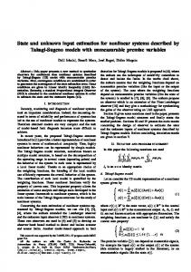
Our basic idea is to test the performance of the different versions of DHF for a high dimensional, non-linear, nonGaussian system. Numerical results for the DHF have been mentioned in [17] and [12]. We find two other sources who have picked up on DHF and have tried to implement. First, DHF based on the incompressible flow and ZDEF have been implemented by Choi. et.al. in [16] for a non-linear Scaler and a linear vector system models. Particles are generated by sampling the transition density. An EKF/UKF is run in parallel to the main algorithm. This is done in order to approximate the prior covariance matrix. Hence there is performance dependency of DHF on the EKF/UKF. It has been reported that the ZDEF-DHF performs superior to the incompressible flow filter, EKF, UKF and achieve better accuracy than a standard particle filter with fewer particles. We call this implementation as the original ZDEF-DHF. The second implementation of the ZDEF-DHF has been reported by Ding and Coates in [19], and a pseudo-code is also provided. Make two distinct changes are made to the original ZDEF-DHF. In the first modification the linearization of the measurement equation is carried out for individual particles, as opposed to being done only at the prior mean location. The second modification is related to the feedback of the DHF state estimates to the EKF, making the filters coupled. In this study we consider two cases, 1) the first modification alone and 2) with the feedback. We call these implementations as modified ZDEF-DHF and modified ZDEFDHF-FB respectively. As per our knowledge, no results have yet been published for the NZDCF-DHF. The implementation for the NZDCF-DHF is done on the same lines as for the modified ZDEF-DHF (without feedback). We simulate four targets (N =4) in our analysis. ∆t is set 3 2 to 1, σa2 to 50 ms−2 , σr2 is set to 10000m2 , σr2x to 10 σr , while 2 1 2 β is set to 10 rad . Since the process and measurement noises have high covariance and the bearing noise is assumed to be non-Gaussian, the state estimation becomes quite challenging. In particular we note that σr < Di,k σθ ∀i, k, where Di,k represents the distance of ith target from the radar location at time instant k. Three sets of coupling constants {κ1 , κ2 and κ3 } are used, {0,0,0}, {100, 0.005, 0.005} and {8000, 0.05, 0.1}. First set refers to an un-coupled model, second to a weakly coupled while and the third to a strongly coupled model as shown in figures 1a, 1b and 1c respectively. The turn radius rt and turn speed vt are set to 200 m and 10 ms−1 while δ is set to 0.001. Targets position element are initialized by sampling Gaussian distribution with mean

of 20000 m and variance of 5000 m2 , while the velocity elements from Gaussian distribution with mean and variance of 100 m and 100 m2 respectively. EKF is initialized by sampling the Gaussian with initial state vector as mean and with variances 105 and 1 for the position and the velocity respectively. Particles are draw for DHF and BPF in a similar way. The discretization of pseudo-time λ is critical for the filters performance. As stated in [14], the incompressible flow and ZDEF- DHF can implemented with uniform step size ∆λ = 0.1 but not for NZDCF-DHF. For comparison between the two flows, we plot the average of the flow vector norm Np ∑ 1 |f (xi , λ)| against λ for both ZDEF and NZDCF, in the Np i=1

case of the strongly coupled motion. Here the averaging is done across the number of particles (Np ), 5

10

ZDEF NZDCF

Ave. flow vector norm.

traditional solutions like the EKF and the Particle filter. The likelihood function can be written as in equation (D3).

4

10

3

10

2

10

1

10 −3 10

−2

−1

10

10

0

10

λ

Fig. 2: Log homotopy based flow vs. λ We note that the normed averaged ZDEF starts around 5000 and is fairly smooth, exhibiting an order of magnitude change in the interval between 10−3 and 1. On the other hand the NZDEF is much more dynamic and an approximately three order of magnitude change can be observed in the same interval. This implies that, if the flow is coarsely sampled, say uniformly with ∆λ = 0.1, the loss in performance for NZDCF-DHF can be far greater than for ZDEF-DHF as the flow dynamics would not be captured sufficiently well. One the other hand, a very fine λ discretization can lead to an increased computational cost. Therefore, in this work we choose a middle ground and use 39 exponentially spaced λ points between 0 and 1, as recommended in [14]. We use root average mean square error (RAMSE) as the performance metric. It is defined as following. Let M be the total number of simulation runs for a particular scenario, xi,m k and yki,m denote the positions of the ith target along X and Yaxis respectively, at time instant k in the mth trial. Likewise, let x ˆi,m and yˆki,m denote estimated positions for the ith target. k

The RAMSE εd is then defined as, v ] [ d ( u M )2 ( )2 ) u 1 ∑ 2 ∑ ( i,m i,m i,m i,m t εd = xk − x ˆk + yk − yˆk M m=1 d i=1 (19) In figure 3, we plot the RAMSE(εd ) for the target positions as a function of time for the EKF , different versions of DHF (Np = 100) and BPF with 104 and 2.5×104 particles, averaged over fifty simulation runs (M = 50). There are three figures, one each for the un-coupled, weakly coupled and strongly coupled models. 16000

εd [m]

12000

EKF Original ZDEF−DHF Modified ZDEF−DHF Modified ZDEF−DHF−FB NZDCF−DHF 5

BPF(N = 2.5 x 10 ) 8000

5

BPF(N = 10 )

4000

0

20

40

60

80

100

Time [s] (a) 16000

εd [m]

12000

EKF Original ZDEF−DHF Modified ZDEF−DHF Modified ZDEF−DHF−FB NZDCF−DHF BPF(N = 2.5 x 105)

8000

BPF(N = 105)

4000

0

V. 20

40

60

80

100

80

100

Time [s] (b) 16000

εd [m]

12000

EKF Original ZDEF−DHF Modified ZDEF−DHF Modified ZDEF−DHF−FB NZDCF−DHF BPF(N = 2.5 x 105)

8000

BPF(N = 105)

4000

0

NZDCF-DHF has the lowest RAMSE amongst all version of DHF. In particular, Original ZDEF-DHF has the worst performance. The BPF with 10000 and 25000 particles have almost similar performance. It can be noted that the error is generally high for all filters. This can be attributed to the use of high values of process and measurement noise covariances. For the weakly coupled model, targets trajectories are loosely interdependent. RAMSE for DHF/EKF start diverging earlier in this case. Again, we note that the BPF are the best performers, filter with 25000 particles having a slightly better performance. NZDCF-DHF outperforms all other versions of the DHF and the EKF as before but is beaten by the BPF. Actually in this case the difference in the εd between the BPF and NZDCFDHF is higher. At last we discuss the strongly coupled model. Here, the pursuing targets tightly follow the lead target. This might lead to a rapid change in the direction and speed, which coupled with high noise covariances can lead to worse estimation of targets positions. We observe quite significant difference in the performance of different DHF variants. All DHF variants except the NZDCF-DHF, perform even worse than the EKF. The modified ZDEF-DHF-FB has the worst performance. The NZDCF-DHF, even tough better than other DHF and EKF, still does not outperform the BPF. Next we compare the execution time τexec for a single recursion, including both the time and the measurement update steps. Simulations were performed on the computer with Intel Core2 Quad with 2.66 GHz processors and 4 GB RAM. The τexec was 0.0005s for EKF, 0.011s for original ZDEF-DHF , 0.75s for modified ZDEF-DHF, 1.43s for NZDCF-DHF, and 1.16s and 4.34s for BPF with 10000 and 25000 particles. The main requirement for the NZDCF-DHF is that the log p(x, λ) is no-where vanishing, twice differentiable and with a nonsingular hessian matrix [14]. These requirements are met in our case.

20

40

60

Time [s] (c)

Fig. 3: Dimension-free error for (a) un-coupled , (b) weakly coupled and (c) strongly coupled model. First we discuss the uncoupled model. All targets move independently of each other. We observe that until 30s, εd for all filters grow almost linearly. After that the εd for EKF and ZDEF-DHF grow faster than that of BPF and NZDCF-DHF.

D ISCUSSION

We have seen that the DHF performance, even though better than the EKF, is still not superior to the BPF with similar execution time. There could be several reasons for this particular behavior. That includes the theoretic considerations e.g. approximations made while deriving the flow solutions, and the implementation aspects like the use of relatively simple Euler’s integration method for numerically solving the flow equation etc. Also, DHF particles are sampled from p(xk+1 |xk ) just like in a BPF. A better choice of the importance density could lead to the better estimation. The idea of importance sampling with a particle flow has been used in [20], where filtered particles are not directly used for the evaluation of the point estimates. Instead, they are considered as samples from an importance density and hence are assigned weights. This allows for the corrections of the approximation errors. In the case of high weight variance, a MCMC step can also be used. Finally, the performance of all DHF variants depends on the accuracy of the prior covariance matrix estimation. In the current work, it is obtained from a parallel running EKF. A better approximation to the prior covariance matrix estimation might also improve the estimation accuracy. VI.

C ONCLUSION

We have studied the state estimation of a coupled, nonlinear and non-Gaussian system model using DH filters. Sev-

eral versions of DHF exist, that have been derived based on different sets of assumptions. Estimates from a parallel running EKF/UKF is used to approximate the prior covariance matrix. Different degrees of coupling in the dynamic model leads to different results. Though NZDCF-DHF performs better than all other versions of DHF and the EKF, it is outperformed by the BPF with the same order of execution time. The difference in the performance is greatest when the motion of the targets is strongly coupled. Improved performance for NZDCF-DHF can be expected with the increase in the number of particles, better estimates for the prior covariance matrix and importance weighting of the particles. Also adaptive psuedo time discretization can help in reducing the execution time. R EFERENCES [1] [2]

[3]

[4]

[5]

[6]

F. Gustafsson, Statistical sensor fusion. Studentlitteratur, 2010. M. Arulampalam, S. Maskell, N. Gordon, and T. Clapp, “A tutorial on particle filters for online non-linear/ non-gaussian bayesian tracking,” in IEEE transaction on signal processing, vol. 50, no. 2. IEEE, February 2002, pp. 174–188. N. Gordon, D. Salmond, and A. Smith, “Novel approach to nonlinear/non-gaussian bayesian state estimation,” in IEE Proceedings on Radar and Signal Processing., Apr 1993, pp. 107–113. M. Pitt and N. Shephard, “Filtering via simulation: Auxiliary particle filters,” in Journal of the American Statistical Association, vol. 94, no. 446, 1999. C. Musso, N. Oudjane, and F. Le Gland, “Improving regularised particle filters,” in Sequential Monte Carlo Methods in Practice, ser. Statistics for Engineering and Information Science, A. Doucet, N. de Freitas, and N. Gordon, Eds. Springer New York, 2001, pp. 247–271. U. Hanebeck and O. Feiermann, “Progressive bayesian estimation for nonlinear discrete-time systems: the filter step for scalar measurements and multidimensional states,” in IEEE Conference on Decision and Control, vol. 5. IEEE, 9-12 Dec. 2003, pp. 5366–5371.

[7] J. Hagmar, M. Jirstrand, L. Svensson, and M. Morelande, “Optimal parameterization of posterior densities using homotopy,” in Proceedings of the 14th International Conference on Information Fusion (FUSION). 5-8 July: IEEE, 2011, pp. 1–8. [8] F. Daum and J. Huang, “Curse of dimensionality and particle filters,” in IEEE Aerospace conference. IEEE, 8-15 March 2003, pp. 1970–1993. [9] F. Daum and J. Huang, “Nonlinear filters with log-homotopy,” in SPIE Proceedings, September 2007. [10] F. Daum and J. Huang, “Nonlinear filters with particle flow,” in SPIE Proceedings, September 2009. [11] F. Daum and J. Huang, “Nonlinear filters with particle flow induced by log-homotopy,” in SPIE Proceedings, May 2009. [12] F. Daum, J. Huang, and A. Noushin, “Coulomb’s law particle flow for nonlinear filters,” vol. 8137, 2011, pp. 81 370E–81 370E–15. [13] F. Daum and J. Huang, “Zero curvature particle flow for nonlinear filters,” in SPIE Proceedings, 2013. [14] F. Daum and J. Huang, “Particle flow with non-zero diffusion for nonlinear filters,” in SPIE Proceedings, 2013. [15] F. Daum and J. Huang, “Particle flow for nonlinear filters with loghomotopy,” in SPIE Proceeding, April 2008. [16] S. Choi, P. Willet, F. Daum, and J. Huang, “Discussion and application of homotopy filter,” in SPIE Proceedings, 2011. [17] F. Daum and J. Huang, “Numerical experiments on nonlinear filters with exact particle flow induced by log-homotopy,” in Proceeding SPIE, April 2010. [18] F. Daum and J. Huang, “Generalized particle flow for nonlinear filters,” in SPIE Proceeding, April 2010. [19] T. Ding and M. Coates, “Implementation of daum-huang exact flow particle filter,” in IEEE Statistical Signal Processing Workshop (SSP), 2012. [20] P. Bunch and S. Godsill, “Approximations of the optimal importance density using gaussian particle flow importance sampling,” Tech. Rep., 2014.