dissertation asks and answers the question: \Can we do better?" ..... A neural network can be de ned as a set of nodes (neurons) each of which has an ..... We can get the same a ect by permanently clamping an auxiliary input to the .... where is, once again, the learning rate, and E is a quadratic error function de ned as. E =.
Nonmonotonic Activation Functions in Multilayer Perceptrons Gary William Flake Institute for Advance Computer Studies Department of Computer Science University of Maryland College Park, MD 20742
Acknowledgement: This work was partially supported by AFOSR grant number F49620-92-J-0519.
Abstract Title of Dissertation: Nonmonotonic Activation Functions in
Multilayer Perceptrons
Gary William Flake, Doctor of Philosophy, 1993 Dissertation directed by: Professor Yee-Chun Lee Professor James A. Reggia Department of Computer Science Multilayer perceptrons (MLPs) and radial basis function networks (RBFNs) are the two most common types of feedforward neural networks used for pattern classi cation and continuous function approximation. MLPs are characterized by slow learning speed, low memory retention, and small node requirements, while RBFNs are known to have high learning speed, high memory retention, but large node requirements. This dissertation asks and answers the question: \Can we do better?" Two types of neural network architectures are introduced: the hyper-ridge and the hyper-hill. A hyperridge network is a perceptron with no hidden layers and an activation function in the form g(h) = sgn(c2 ? h2 ) (h is the net input; c is a constant \width"), while a hyper-hill network is a continuous multilayer version with g(h) = exp(?h2 =c2). Throughout this dissertation theoretical and empirical evidence is presented which strongly indicates that hyper-hills behave similarly to MLPs when the input dimension is large but are more similar to RBFNs when the input dimension is low. Additionally, the fact that hyper-hills learn faster than MLPs and require fewer nodes, but do not su�er the \curse of dimensionality" associated with RBFNs, is o�ered as evidence that hyper-hills ll a niche between MLPs and RBFNs.
Nonmonotonic Activation Functions in Multilayer Perceptrons by Gary William Flake Dissertation submitted to the Faculty of the Graduate School of The University of Maryland in partial ful llment of the requirements for the degree of Doctor of Philosophy 1993
Advisory Committee: Professor James A. Reggia, Chairman / Co-Advisor Associate Professor William Gasarch Professor Laveen Kanal Professor Yee-Chun Lee, Co-Advisor Professor Dianne O'Leary
c Copyright by
Gary William Flake 1993
Contents List of Tables List of Figures 1 Introduction
1.1 Neural Networks : : : : : : : : : : : : : : : : : : : : : : : : : : : : : : : : : : : : : : : : : : : 1.2 Contributions : : : : : : : : : : : : : : : : : : : : : : : : : : : : : : : : : : : : : : : : : : : : : 1.3 Overview : : : : : : : : : : : : : : : : : : : : : : : : : : : : : : : : : : : : : : : : : : : : : : :
2 Background
2.1 Simple Perceptrons : : : : : : : : : : : : : : : : : : 2.1.1 Simple Perceptron Learning : : : : : : : : : 2.1.2 Basic Results : : : : : : : : : : : : : : : : : 2.2 Multilayer Perceptrons : : : : : : : : : : : : : : : : 2.2.1 MLP Forward Dynamics : : : : : : : : : : : 2.2.2 The Backpropagation Learning Algorithm : 2.2.3 Features of MLPs : : : : : : : : : : : : : : 2.3 Radial Basis Function Networks : : : : : : : : : : : 2.3.1 A Simple RBFN : : : : : : : : : : : : : : : 2.3.2 Extensions : : : : : : : : : : : : : : : : : : 2.3.3 Features of RBFNs : : : : : : : : : : : : : : 2.4 Nonmonotonic Activation Functions : : : : : : : :
3 Hyper-Ridge Representation 3.1 3.2 3.3 3.4
The Hyper-Ridge Network : : : : : : : : : : : Linear Inseparability : : : : : : : : : : : : : : The Representation Power of a Hyper-Ridge : Comparing Representation Power : : : : : : :
4 Hyper-Ridge Learning 4.1 4.2 4.3 4.4 4.5
The Hyper-Ridge Learning Algorithm Examples : : : : : : : : : : : : : : : : The Geometry of the Solution-Space : Local Convergence : : : : : : : : : : : Weight Oscillations : : : : : : : : : : :
5 Hyper-Hills
5.1 Overview : : : : : : : : : : 5.2 Emulation : : : : : : : : : : 5.3 Error Bounds on Emulation 5.3.1 Overview : : : : : :
: : : :
: : : :
: : : :
: : : :
: : : :
: : : :
: : : : : : : : : : : :
: : : : : : : : : : : :
: : : : : : : : : : : :
: : : : : : : : : : : :
: : : : : : : : : : : :
: : : : : : : : : : : :
: : : : : : : : : : : :
: : : : : : : : : : : :
: : : : : : : : : : : :
: : : : : : : : : : : :
: : : : : : : : : : : :
: : : : : : : : : : : :
: : : : : : : : : : : :
: : : : : : : : : : : :
: : : : : : : : : : : :
: : : : : : : : : : : :
: : : : : : : : : : : :
: : : : : : : : : : : :
: : : : : : : : : : : :
: : : : : : : : : : : :
: : : : : : : : : : : :
: : : : : : : : : : : :
: : : : : : : : : : : :
: : : : : : : : : : : :
: : : :
: : : :
: : : :
: : : :
: : : :
: : : :
: : : :
: : : :
: : : :
: : : :
: : : :
: : : :
: : : :
: : : :
: : : :
: : : :
: : : :
: : : :
: : : :
: : : :
: : : :
: : : :
: : : :
: : : :
: : : :
: : : :
: : : :
: : : : :
: : : : :
: : : : :
: : : : :
: : : : :
: : : : :
: : : : :
: : : : :
: : : : :
: : : : :
: : : : :
: : : : :
: : : : :
: : : : :
: : : : :
: : : : :
: : : : :
: : : : :
: : : : :
: : : : :
: : : : :
: : : : :
: : : : :
: : : : :
: : : : :
: : : : :
: : : : :
: : : : :
: : : : :
: : : : :
: : : : :
: : : :
: : : :
: : : :
: : : :
: : : :
: : : :
: : : :
: : : :
: : : :
: : : :
: : : :
: : : :
: : : :
: : : :
: : : :
: : : :
: : : :
: : : :
: : : :
: : : :
: : : :
: : : :
: : : :
: : : :
: : : :
: : : :
: : : :
: : : :
: : : :
: : : :
: : : :
ii
iv v 1 1 2 4
6
6 7 8 8 8 10 11 12 12 14 15 15
18 18 19 20 25
33 33 34 36 39 41
48 48 50 52 53
5.3.2 Background : : : : : : 5.3.3 Gaussian Equivalence 5.4 Hyper-Hill Learning : : : : : 5.5 Di�cult Representations : : : 5.6 Summary : : : : : : : : : : :
: : : : :
: : : : :
: : : : :
: : : : :
: : : : :
: : : : :
: : : : :
: : : : :
: : : : :
: : : : :
: : : : :
: : : : :
: : : : :
: : : : :
: : : : :
: : : : :
: : : : :
: : : : :
: : : : :
: : : : :
: : : : :
: : : : :
: : : : :
: : : : :
: : : : :
: : : : :
: : : : :
: : : : :
: : : : :
6.1 The MONK's Problems : : : : : : : : : : : 6.1.1 Previous Results : : : : : : : : : : : 6.1.2 Hyper-Hill Results : : : : : : : : : : 6.1.3 Why Do Hyper-Hills Work So Well? 6.2 The Mackey-Glass Equation : : : : : : : : : 6.3 Summary : : : : : : : : : : : : : : : : : : :
: : : : : :
: : : : : :
: : : : : :
: : : : : :
: : : : : :
: : : : : :
: : : : : :
: : : : : :
: : : : : :
: : : : : :
: : : : : :
: : : : : :
: : : : : :
: : : : : :
: : : : : :
: : : : : :
: : : : : :
: : : : : :
: : : : : :
: : : : : :
: : : : : :
: : : : : :
: : : : : :
: : : : : :
: : : : : :
: : : : : :
: : : : : :
: : : : : :
6 Empirical Results
: : : : :
: : : : :
: : : : :
: : : : :
: : : : :
: : : : :
: : : : :
54 55 57 58 62
64 64 65 66 68 69 74
7 Conclusion
75
Bibliography
77
7.1 Summary : : : : : : : : : : : : : : : : : : : : : : : : : : : : : : : : : : : : : : : : : : : : : : : 75 7.2 Limitations : : : : : : : : : : : : : : : : : : : : : : : : : : : : : : : : : : : : : : : : : : : : : : 76 7.3 Future Work : : : : : : : : : : : : : : : : : : : : : : : : : : : : : : : : : : : : : : : : : : : : : 76
iii
List of Tables 1.1 Comparison Between Local and Global Mappings : : : : : : : : : : : : : : : : : : : : : : : : :
2
2.1 Summary of MLP Feedforward Notation : : : : : : : : : : : : : : : : : : : : : : : : : : : : : : 9 2.2 Summary of RBFN Feedforward Notation : : : : : : : : : : : : : : : : : : : : : : : : : : : : : 12 3.1 Comparison of Number of Hyper-Ridge and Perceptron Dichotomies : : : : : : : : : : : : : : 25 4.1 Negate | Weights : : : : : : : : : : : : : : : : : : : : : : : : : : : : : : : : : : : : : : : : : : 34 4.2 Symmetry | Weights : : : : : : : : : : : : : : : : : : : : : : : : : : : : : : : : : : : : : : : : 35 4.3 Count(3) | Weights : : : : : : : : : : : : : : : : : : : : : : : : : : : : : : : : : : : : : : : : : 36 5.1 Summary of Hyper-Hill Feedforward Notation : : : : : : : : : : : : : : : : : : : : : : : : : : : 49 6.1 6.2 6.3 6.4
MONK's Problems Results for Other Techniques : : : : MONK's I, II, & II Results for Hyper-Hill : : : : : : : : MONK's III Results for Hyper-Hill with Weight Decay : MONK II Weights from Hyper-Hill : : : : : : : : : : : :
iv
: : : :
: : : :
: : : :
: : : :
: : : :
: : : :
: : : :
: : : :
: : : :
: : : :
: : : :
: : : :
: : : :
: : : :
: : : :
: : : :
: : : :
: : : :
: : : :
: : : :
: : : :
66 67 67 68
List of Figures 1.1 Mapping Structures in One and Two Dimensions : : : : : : : : : : : : : : : : : : : : : : : : :
3
2.1 One solution for the XOR Mapping : : : : : : : : : : : : : : : : : : : : : : : : : : : : : : : : :
9
3.1 3.2 3.3 3.4 3.5 3.6 3.7 3.8 3.9 3.10 3.11
A Hyper-Ridge and Hyperstep In Two Dimensions : : Hyper-Ridge Networks to Compute Various Mappings Hyper-Ridge Dichotomy in One Dimension : : : : : : Two Dichotomies of Four Points in a Plane : : : : : : Projecting Dichotomies Onto one Lower Dimension : : Dp (p; d)=2p Versus p=(d + 1) for Various Values of d : Dh (p; d)=2p Versus p=(d + 1) for Various Values of d : Capacity Comparison for d = 5 : : : : : : : : : : : : : Capacity Comparison for d = 20 : : : : : : : : : : : : Capacity Comparison for d = 100 : : : : : : : : : : : : Dh (p; d)=Dp(p; d) Versus p for Various Values of d : :
: : : : : : : : : : :
: : : : : : : : : : :
: : : : : : : : : : :
: : : : : : : : : : :
: : : : : : : : : : :
: : : : : : : : : : :
: : : : : : : : : : :
: : : : : : : : : : :
: : : : : : : : : : :
: : : : : : : : : : :
: : : : : : : : : : :
: : : : : : : : : : :
: : : : : : : : : : :
: : : : : : : : : : :
: : : : : : : : : : :
: : : : : : : : : : :
: : : : : : : : : : :
: : : : : : : : : : :
: : : : : : : : : : :
: : : : : : : : : : :
: : : : : : : : : : :
: : : : : : : : : : :
19 19 21 22 22 27 27 28 28 29 29
4.1 4.2 4.3 4.4 4.5 4.6
Regions in Weight-Space With No Solutions : : : : : : The Error Surface : : : : : : : : : : : : : : : : : : : : Zoom of the Error Surface : : : : : : : : : : : : : : : : A Global Minima : : : : : : : : : : : : : : : : : : : : : A Local Minima : : : : : : : : : : : : : : : : : : : : : Equivalence of Hyper-Ridges and a Subclass of MLPs
: : : : : :
: : : : : :
: : : : : :
: : : : : :
: : : : : :
: : : : : :
: : : : : :
: : : : : :
: : : : : :
: : : : : :
: : : : : :
: : : : : :
: : : : : :
: : : : : :
: : : : : :
: : : : : :
: : : : : :
: : : : : :
: : : : : :
: : : : : :
: : : : : :
: : : : : :
37 44 44 45 45 46
5.1 5.2 5.3 5.4 5.5 5.6 5.7 5.8 5.9 5.10 5.11 5.12
Two Possible Activation Functions for a Hyper-Hill : : : : : : : : : : Translating Sigmoids Into Gaussian-like Functions : : : : : : : : : : A Single Hyper-Hill : : : : : : : : : : : : : : : : : : : : : : : : : : : : Two Hyper-Hills Added Together : : : : : : : : : : : : : : : : : : : : Two Hyper-Hills Added Together And Composed Through A Third The Activation Function and First Derivative : : : : : : : : : : : : : Output Response of a 2-1 Hyper-Hill for the OR function : : : : : : Output Response of an Over-Trained 2-1-1 Hyper-Hill : : : : : : : : Output Response of an Over-Trained 2-2-1 Hyper-Hill : : : : : : : : Output Response of a Properly Trained 2-1-1 Hyper-Hill : : : : : : : Output Response of a Properly Trained 2-2-1 Hyper-Hill : : : : : : : Output Response 2-2-1 Hyper-Hill with Weight Decay : : : : : : : :
: : : : : : : : : : : :
: : : : : : : : : : : :
: : : : : : : : : : : :
: : : : : : : : : : : :
: : : : : : : : : : : :
: : : : : : : : : : : :
: : : : : : : : : : : :
: : : : : : : : : : : :
: : : : : : : : : : : :
: : : : : : : : : : : :
: : : : : : : : : : : :
: : : : : : : : : : : :
: : : : : : : : : : : :
: : : : : : : : : : : :
49 50 51 51 51 57 59 60 60 61 61 62
6.1 6.2 6.3 6.4 6.5
Hyper-Hill Prediction Results For MG Train Set Hyper-Hill Error Results For MG Train Set : : : Hyper-Hill Prediction Results For MG Test Set : Hyper-Hill Error Results For MG Test Set : : : : Comparison of Techniques on the MG Test Set :
: : : : :
: : : : :
: : : : :
: : : : :
: : : : :
: : : : :
: : : : :
: : : : :
: : : : :
: : : : :
: : : : :
: : : : :
: : : : :
: : : : :
70 70 71 71 72
v
: : : : :
: : : : :
: : : : :
: : : : :
: : : : :
: : : : :
: : : : :
: : : : :
: : : : :
: : : : :
: : : : :
6.6 Training Time Versus Prediction Error : : : : : : : : : : : : : : : : : : : : : : : : : : : : : : : 73
vi
Chapter 1
Introduction Researchers in the computational sciences have long known that the human brain is vastly superior to the digital computer in solving many interesting problems. To illustrate this, consider the typical tasks performed by any three year old child. A child can recognize human faces, understand and speak sentences in her native language, maneuver a tricycle e�ciently through a room of obstacles, and manipulate objects with her hands in an arbitrary manner. Moreover, most children can do, and often do, all of these things simultaneously. By way of comparison, the most advanced computers in existence can only perform these tasks in a very simpli ed manner. On the other hand, digital computers can manipulate, store, and retrieve binary symbols with blinding speed and accuracy. In fact, a single human neuron is rather slow and clumsy when compared to the typical pocket calculator. However, the real power of the human brain lies in the massive parallelism that exists within it. With 1011 neurons and 1013 to 1014 synapses connecting the neurons, the human brain is able to process vast amounts information in such a way as to make the most challenging computational tasks seem trivial. To get computers to operate in a more powerful manner researchers have used neuroscience as a starting place for designing new types of computing machines. An arti cial neural network is one realization of brain inspired devices.
1.1 Neural Networks There are many di�erent types of neural models used by researchers to solve interesting problems. Despite this fact, all of these models have some common features that allow us to discuss functionality and structure on equal footing. A neural network can be de ned as a set of nodes (neurons) each of which has an activation value, a set of connection weights (synapses) which connect the nodes, a propagation rule which determines the net input values into each of the nodes, and an activation rule which computes a node's activation value based on its net input value. The important part of this description is that all of the computations performed are local at each node. The emergent behavior of the entire neural network is determined by the behavior of each of the nodes which in turn act as independent units | each performs a function that is largely independent of the other units. This is similar in spirit to other highly parallel systems such as an ant colony, immune systems, the global economy, cellular automata, genetic evolution, and the weather. The propagation rule of a neural network, which maps many real valued inputs into a single real output, is more rigorously de ned as a function, h : 0. Note that this simply speci es that w must de ne a hyperplane such that all positive target patterns fall to one side of the hyperplane, and all negative patterns fall to the other side. In fact, this is the essence of the result that simple perceptrons can only represent functions that are linearly separable, since if no such hyperplane exists then a perceptron cannot represent the mapping.
2.1.1 Simple Perceptron Learning
If a pattern set can be decided by a simple perceptron, then the perceptron learning algorithm can be used to determine a weight vector that will correctly classify all of the patterns. The procedure iterates through the entire training set and picks a pattern which is incorrectly classi ed. This pattern is then used to update the weight vector with the rule wt+1 = wt + �w; (2:7) where t is used as a time or iterate index. The term �w can be de ned as �w = �t� x�
(2:8)
when updates are only made if the pattern is misclassi ed, or (2:9) �w = 21 �(t� ? y� )x� if we wish to update the weight vector at all times. In both cases � plays the role of a step size or learning rate. Equation 2.8 is reminiscent of Hebbian learning in that an update is made proportional to the product of the input and target values. Equation 2.9 is similar in spirit to gradient based techniques (which will be discussed in the next section); however, since the activation function, g(h), is not continuous, there is no true gradient based algorithm to use in this case. In any event, the perceptron learning algorithm is typically referred to as the delta rule. 1 The expression (w x) is to be interpreted as the inner product operation. I am omitting the transpose operator to avoid con icting with superscript indices that will be used later. �
7
2.1.2 Basic Results
The two most important questions that have been asked about simple perceptrons are: � Under what set of circumstances can one expect the perceptron learning algorithm to nd a solution weight vector for a pattern set? � Since perceptrons can only represent mappings that are linearly separable, and a classi cation problem can be viewed as \coloring" an input pattern set, how many random input-output pattern sets can one expect to color? For the rst question, the perceptron convergence theorem guarantees that if there exists a solution then the perceptron learning algorithm will always converge in a nite number of steps [50, 36]. As for the second question, let C represent the capacity of a perceptron, which is the maximum number of random patterns that one can expect to store in a simple perceptron with one output which takes binary values. Since the number of weights in the perceptron is linear in the number of inputs, d, we should expect C to be a function of d. Cover [11], Nilsson [40], and Gardner [21] have all shown that C = 2(d + 1) for a simple perceptron with a bias term, and C = 2d for a perceptron with no bias terms. The above rules should be interpreted as saying that if one attempted to store more than C patterns in a perceptron then the performance would degrade at least by the amount that the actual number of patterns exceeds C.
2.2 Multilayer Perceptrons The most obvious drawback of a single layer perceptron is its inability to represent linearly inseparable mappings. It has long been known that perceptrons with a \hidden" layer of nodes are capable of overcoming this shortcoming, but it took more than a decade to discover a learning algorithm that could train a continuous multilayer perceptron to learn anything. Contrary to a common misconception that Rosenblatt was ignorant of this shortcoming, a discussion of the di�culty with representing linearly inseparable problems can be found in [50].2 Minsky and Papert, besides explicitly pointing out that whole classes of mappings could not be represented by simple perceptrons, gave some attention to Gamba machines [36], which are very similar to the multilayer perceptrons used today. Consider the simple binary function XOR.3 The XOR mapping is linearly inseparable since no single hyperplane can divide the input patterns into the proper sets.4 However, OR, AND, and NAND, as well as all other two input binary functions, are readily computable by a simple perceptron. Since x y = (x _ y) ^ :(x ^ y); a perceptron with two inputs, two hidden nodes, one output, and complete forward connectivity between nodes in adjacent layers can trivially compute the desired function. Figure 2.1 illustrates such a perceptron. On the left are the hyperplanes to compute NAND (vertical lines) and OR (horizontal lines). The intersection of the two regions properly isolates the two sets in the XOR mapping. On the right is a two layer perceptron that implements the XOR mapping. The connection weights are shown next to each arc, and a bias value is indicated in the node itself. The left hidden node in the perceptron implements the OR function, while the right hidden node implements NAND. The output node implements the AND of the results of the hidden nodes, thus computing the correct mapping for XOR.
2.2.1 MLP Forward Dynamics 2 Moreover, Rosenblatt also discovered the \back-propagating error correction procedure" which is a probabilistic, discrete, learning algorithm to train all connection weights of a multilayer, discrete perceptron. 3 XOR is de ned for binary values; thus, values of -1 play the role of 0 when using activation functions with a range of [-1, 1]. 4 The negation of XOR, EQUALITY, has the same feature.
8
AND
1 1
OR
1
-1 1
-1 1
-1
NAND
-1
Figure 2.1: One solution for the XOR Mapping Table 2.1: Summary of MLP Feedforward Notation ali bli hli wijl g(h) L
: : : : : :
nl n yi xi
: : : :
activation level of node i in node layer l bias value of node i in node layer l net input of the node i in node layer l connection weight from alj?1 to node i in layer l sigmoidal activation function the number of weight layers in a network, and the index for the last layer the number of nodes in layer l the number of network outputs, nL synonym for the ith network output and aLi synonym for the ith network input and a0i
Since we are now dealing with multilayer neural networks, the notation used in the previous section is insu�cient. In this and all future sections, an l layer network will be understood as meaning a network with l + 1 layers of nodes (including the input layer) and l layers of connection weights between each node layer. Additionally, the rst node layer (the inputs) will be indexed by 0, with the rst weight layer being indexed by 1, while the last node layer is indexed by L for the generic case when the number of layers is unspeci ed. When in doubt, consult Table 2.1, which contains a summary of the notation used in this section. With this in mind, we can de ne the forward dynamics for a single node layer of a multilayer perceptron as 1 0nl?1 X (2:10) ali = g(hli ) = g @ wijl ajl?1 ? bli A j =1
where superscripts are now used to indicate the layer, and nl is the number of nodes in the lth node layer. Alternately, Equation 2.10 can be expressed in vector notation as
?
�
al = g(hl) = g Wl al? ? bl : 9
1
(2:11)
For a simple perceptron, g(h) took the form of a step function. To derive the learning algorithm for a continuous multilayer perceptron we will need the activation function to be di�erentiable and, therefore, continuous. The hyperbolic tangent function g(h) = tanh(h); or the logistic function
g(h) = (1 + exp(?h))?1 are both good approximations to a step function and satisfy our di�erentiable requirement. In keeping with previous sections, I will use the hyperbolic tangent, since its range is [-1, 1]. To compute the output of a multilayer perceptron we apply Equation 2.10 (or Equation 2.11) to each node layer but the rst, starting with the rst layer above the inputs and ending with the outputs.
2.2.2 The Backpropagation Learning Algorithm
Now that we know that a multilayer perceptron can represent an XOR mapping, how would one go about teaching the perceptron to duplicate the mapping? The problem here is that the delta rule says nothing about hidden nodes. In fact, it only speci es weight changes for the outermost layer of weights when a target value is known. If one knew the correct responses for a hidden node then one could train the hidden nodes on some target value as is done for output nodes. However, if this is true, then the problem is already largely solved. To solve this problem, the backpropagation learning algorithm was discovered independently by a number of researchers [7, 63, 52]. The main feature of the learning algorithm is to replace the discrete activation function with a continuous, monotonicly increasing function and to derive the update rules for the weight changes based on gradient descent. Thus, in the update equation
wt = wt + �w; +1
we de ne
�w = ?� @@E w where � is, once again, the learning rate, and E is a quadratic error function de ned as n X E = 21 (ti ? yi )2 : i=1
(2:12) (2:13)
For every weight in every layer, we can compute the gradient of the error function with respect to each weight by application of the chain rule, yielding @E = @E @ali @hli @wijl @ali @hli @wijl @E g0 (hl )al?1 ; (2.14) = @a i j l i where g0 (hli ) is simply the rst derivative of the activation function. Since g(h) = tanh(h), the rst derivative can be expressed as g0(hli ) = (ali ? 1)(ali + 1): (2:15) When l = L (we are looking at the output layer), the rst term in Equation 2.14 is simply @E = @E l (2:16) @ali @yi = yi ? ti = ai ? ti : 10
When l 6= L, the rst term expands to
l+1 @E = nX (2:17) wl+1 @E : @ali j =1 ji @ali+1 Note that this is recursive in the sense that @E=@ai from one layer is computed as a weighted sum of @E=@ai from the layer above it. Combining Equations 2.14, 2.16, and 2.17 into a single learning rule yields ( ?�(al ? t )g0(hl )al?1 when l = L i i i j l �wij = ?� �P (2:18) nl+1 wl+1 @E � g0 (hl )al?1 when l 6= L ; j =1 ji @ali+1 i j
when the actual form of g0 is unknown, and ( ?�(al ? t )(al ? 1)(al + 1)al?1 when l = L i i i i j l �wij = ?� �P nl+1 wl+1 @E � (al ? 1)(al + 1)al?1 when l 6= L ; i i j j =1 ji @ali+1
(2:19)
when g0 is given by Equation 2.15. Equations 2.18 and 2.19 are both known as the backpropagation learning algorithm. The name of the algorithm is appropriate since information is passed backwards though the network. Notice that the backward pass has the same time and memory complexity as the forward pass, since a summation is used in each case. Typically, one trains a network on a pattern set by iterating through each input-output pattern (perhaps randomly) and adjusting the weights after computing the forward and then backward equations. This is known as stochastic or on-line gradient descent. There are several variations on this technique, but they all rely on computing the gradient information in a similar manner.
2.2.3 Features of MLPs
As was illustrated earlier, a single neuron can trivially represent binary functions such as AND and OR. Many classi cation problems can be similarly expressed in terms of set operations (union, and intersection); thus, it is easy to see how one could take a multilayer perceptron and set the weights such that the MLP divides the input-space to decide some complex set mapping. In fact, a MLP is very e�cient at implementing higher dimensional AND and OR functions since it can easily become sensitive or insensitive to an input by making weights extending from an input either large in magnitude or close to zero. The backpropagation learning algorithm is capable of training a MLP on a wide variety of such mappings, yet convergence is never guaranteed. In fact, it is well known that a typical error surface may have many local minima such that an MLP is incapable of learning anything else while also failing to produce the correct responses when trapped in the minima. This is even true when a problem is known to be theoretically solvable. Thus, random initialization of the weights is an important rst step to any learning procedure. Researchers have also used MLPs to approximate continuous function mappings (for example, see Lapedes and Farber [31]). In this case, the output nodes are given a linear activation function, so they may produce output in any range. One can think of this process as forming a decomposition of the input-output space, much like any other decomposition such as a Fourier series. Many have noted that a sigmoid activation function may not be the ideal activation function in this case, since it has global properties which often prove insu�cient in topologically reconstructing an input-output mapping. For example, while a sigmoid's global properties may be a bene t in handling discrete inputs, many continuous functions have local properties such that points distant from one another in the input-space are often completely unrelated and map to very di�erent values. The notion of locality is sometimes di�cult to capture in a function such as a sigmoid. Cybenko and Hornik [12], and Stinchcombe and White [27, 2], have shown that MLPs are universal function approximators on the mapping f : 1).
� For each i > 2 there exists j with i � j � ik and aj 6= 0.
Theorem 5.3.1 di�ers from the corresponding theorem in [13] in one way: in the original form the restriction on the coe�cients was jpij; jqij � 2ki. This turns out to be overly strict. The proof which shows that neural networks with activation function g can �-approximate polynomials relies on a choice of some aN 6= 0 with n � N � nk . Restricting the numerators and denominators to 2poly(i) allows this choice to still be made. Schnitger has con rmed this [55].
Theorem 5.3.2 (DasGupta and Schnitger) A neural network with an activation function g : < ! < and n hidden nodes can approximate the step function over the domain [?1; 1] ? [?2?n; 2?n] with error at most 2?n when
� jg(x) ? g(x + �)j = O(�=x2), for x � 1; � � 0. � 0