NOTE Development of chamber-based sampling technique ... - terrapub

Geochemical Journal, Vol. 41, pp. 493 to 500, 2007

NOTE Development of chamber-based sampling technique for determination of carbon stable isotope ratio of soil respired CO2 and evaluation of influence of CO2 enrichment in chamber headspace YOSHIYUKI TAKAHASHI* and NAISHEN LIANG Center for Global Environmental Research, National Institute for Environmental Studies, 16-2 Onogawa, Tsukuba, Ibaraki 305-8506, Japan (Received April 19, 2007; Accepted September 21, 2007) We developed an experimental method for precise determination of carbon stable isotope ratio (δ13C) of soil-respired CO2 under natural condition. We devised a flask sampling system optimized for collecting soil-respired CO2 to minimize the measurement artifacts related to pressure anomaly. The δ 13C of soil-respired CO2 was estimated from relationship between change rates of the CO2 mole fraction and the δ13C of the CO2 in a closed chamber at the soil surface by using two end-member simple mixing model. We tested the influence of CO2 enrichment in the soil-chamber headspace on the estimates of the δ13C of soil respired CO2 by using high-precision measurements of CO 2 mole fraction and δ13C. To our results, the estimates of the δ13C of soil respired CO 2 was rather insusceptible to the influence of the CO2 enrichment in the chamber as compared with the soil CO2 efflux. Improvement of analytical precision of δ13C is preferred approach to reduce the error in the estimates of δ 13C of soil respired CO2. On the other hand, extending the sampling range of CO2 mole fraction in the chamber can be cost-effective means for the error-reduction practically. Keywords: carbon cycle, soil respiration, stable isotope, atmosphere-terrestrial biosphere exchange, chamber measurement

sphere CO2 exchange. At present circumstances, our primary motivation was to develop methodology and effective measurement strategy for observation of temporal and spatial variations in δ13CR-soil. The main issues in the determination of the δ13CR-soil are how to eliminate measurement artifacts (Högberg et al., 2005). In the present paper, we have defined “soilrespired CO 2 ” as that which diffuses across the soilatmosphere interface and “soil CO2” as the CO 2 found within the soil. The δ 13CR-soil is controlled not only by CO2 produced within the soil but also by diffusion. Under steady-state conditions, δ13CR-soil equals the integrated value of the δ13C produced within the soil, but the δ13C of soil CO2 would be enriched by around 4.4‰ from the δ13CR-soil because of isotopic fractionation during diffusion (Amundsen et al., 1998). Chamber-based measurements can lead to physical disturbance of the CO2 gradient at the soil-atmosphere interface and may thus produce artifacts in the estimation of soil CO 2 efflux (Davidson et al., 2002) and thus, possibly in the estimation of δ 13 CR-soil . In particular, any pressure anomaly would cause mass flow of soil CO2 with an anomalously enriched δ13C value. This effect would lead to artifact in the δ 13CR-soil determination. In addition, alteration of [CO2] in the chamber would change the [CO2] gradient

INTRODUCTION The 13C/12C ratio (commonly expressed in simplified form, δ13C) of atmospheric CO2 provides important information about the carbon budget in global scale (e.g., Tans et al., 1993) and also in ecosystem scale (e.g., Yakir and Sternberg, 2000). Those methods are based on the mass balance of total CO2 and 13CO2 in the atmosphere. Atmospheric CO2 mole fraction ([CO2]) and the δ13C of CO2 both fluctuate within the terrestrial biosphere in response to photosynthetic and respiratory fluxes. Soil respiration is the largest flux component from the terrestrial ecosystem to the atmosphere. Despite its importance, information about temporal and spatial variations in δ 13C of soil respiration (δ 13CR-soil) and its controlling factors under natural condition is lacking because of technical difficulties. Our ultimate goal was to clarify the spatial and temporal distribution of δ13CR-soil in the widespread terrestrial ecosystem. This would ensure functioning of 13C signature as an independent variable to be used in advanced study of atmosphere-terrestrial bio*Corresponding author (e-mail: [email protected]) Copyright © 2007 by The Geochemical Society of Japan.

493

at the soil surface. It would potentially affect the ratio of 13 CO2 to 12CO2 that diffuse across the soil-atmosphere interface, but there is no theoretical analysis available for the effect presently. It should be noted that precise quantification of the magnitude of the bias in the δ 13CR-soil resulted from the measurement artifacts was extremely difficult because of difficulties in accumulating sufficient information at specific times and locations (e.g., vertical distributions of the diffusion coefficient, in situ decomposition rates, and the isotopic composition of the decomposed material). Hence we must carefully plan the field-experiment. The potential problems in the previous sampling techniques had been pointed out in recent studies (e.g., Högberg et al., 2005; Mortazavi et al., 2004; Ohlsson et al., 2005). For example, Flanagan et al. (1996) and Buchmann et al. (1997) collected air in closed chambers into glass flasks during the recovering stage after scrubbing CO 2 by soda lime. This technique would unavoidably involve significant disturbance in CO 2 gradient at soil-atmosphere interface, consequently generated concern for giving influence in isotopic fractionation during diffusion. Ohlsson et al. (2005) tested two different sampling approaches with and without initial flushing of static closed-chamber interior with synthetic air that contained very low CO 2. They reported that lowering of the initial CO2 fraction induced significant enrichment (>4‰) in the δ 13CR-soil. As to the cause of the δ13CR-soil enrichment, the explanation was suggested that the initial lowering of the [CO2] caused a disturbance to the CO2 diffusion process within the soil-chamber system. The experimental configuration of [CO2] gradient for the case of initial-CO2lowering was similar to those of Flanagan et al. (1996), and Buchmann et al. (1997). Ohlsson et al. (2005) also reported that the estimate of δ13CR-soil was not affected by the increase of [CO2] up to more than 2000 µmol·mol–1 for the non-flushed chamber though the apparent CO2 efflux in the chamber was significantly declined. The result suggested that the acceptable [CO 2] range for the δ 13CR-soil determination was larger than that for the determination of soil CO2 efflux. Mortazavi et al. (2004) proposed new field-based sampling approach using open-top-mini-towers. This approach was developed mainly for the precise estimation of δ18O, oxygen stable isotope ratio, of soil respired CO2. But, as for the δ13CR-soil estimation, practical advantage of the approach over the usual closed-chamber sampling was not discussed. Bowling et al. (2003) and McDowell et al. (2004) employed static closed chambers coupled with a flask sampling system for the δ 13CR-soil estimation with consideration for measurement artifacts related to pressure anomaly and to [CO 2 ] enrichment in the chamber headspace. But they did not conduct experimental vali-

494 Y. Takahashi and N. Liang

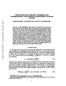
dation of the influence of the [CO2] enrichment. δ13CR-soil has been often estimated from vertical profiles of [CO2] and δ13C of soil CO2 (e.g., Mortazavi et al., 2004; Pendall et al., 2005). This approach assumed that the respiratory end-member δ 13C value was constant with depth. The profiles of soil CO2 and its δ13C were generated from samples collected below the surface soil layer. Hence the estimates by this approach would hardly include the influence of surface litter decomposition (Mortazavi et al., 2004). In seasonal vegetation types like deciduous forest or in tropical ecosystem, decomposition of surface litter contributes largely to the total soil CO2 efflux. Therefore application of this method requires consideration according to the aim of study. Against this background, we developed an air sampling system optimized for the collection of soil-respired CO2 and tested the potential influence from the [CO 2] enrichment in the chamber headspace on the δ13CR-soil estimation by using measurements of [CO2 ] and δ13 C under the natural environment with higher precision than the previous studies. METHODS Field sampling Site description We performed our measurements at the Tomakomai Flux Research site (42°44′ N, 141°31′ E), Japan. The predominant tree species was 45-year-old Japanese larch. The soil was homogeneous and was classified as an immature Volcanogenous Regosol. Automated soil chamber system We employed an alreadyexisting multi-channel automated chamber system for soil CO 2 efflux measurement combined with a newlydeveloped flask sampling system optimized for collecting soil-respired CO2. The automated chamber system was designed to minimize the influence of physical disturbance in soil-atmosphere interface. The details of the chamber system are described by Liang et al. (2003) and Liang et al. (2004). The dimensions of each chamber were 0.9 × 0.9 m, with a height of 0.5 m. The large volume, small vent, and slow movement of the pneumatically actuated lids effectively minimized pressure anomalies inside the chambers during their operation. The flask sampling system described in the following section was located on a wooden slatted drainboard more than 2 m apart from the chambers. The multi-channel automated chamber system was used to monitor [CO2] in the chamber during the flask sampling. Flask sampling system A schematic diagram of the sampling system is shown in Fig. 1. The soil chamber was placed in series in a closed loop with a Mg(ClO4)2 water trap, a diaphragm pump (Model-MOA, GAST Mfg., Inc., Benton Harbor, MI, USA), an assembly of four glass flasks (750-mL, each with two vacuum stopcocks with a

Determination of 13C/12C ratio of soil respired CO2 495

IRGA with Multichannel Sampling System

Vent

Air Flow Meter

Pressure Gauge

M

Back Pressure Regulator

Filter (15mm)

Diaphragm Air Pump

Leak Valve

Filter (2mm)

Flow-mode-A

Fig. 1. Schematic diagram of flask sampling system used in measurements of δ13CR-soil.

Soil Chamber

Sampling line

Sampling line

Mg(ClO4)2 Dryer

Flow-mode-B

Flask

Solenoid valve array

Viton ® O-ring seal at both ends; Koshin Rikagaku Seisakusho, Tokyo, Japan), a back-pressure regulator (Model-6800AL, KOFLOC, Tokyo, Japan), and a flowmeter (Model-RK1000, KOFLOC, Tokyo, Japan). All the glass flasks were connected in series. Solenoid valve arrays (USB3-6-2 and USG3-6-2, CKD, Tokyo, Japan) were placed in parallel with each flask to switch the flow path instantaneously between two modes without stopping the airstream. The airstream bypassed the flasks in flow mode A and passed through the flasks in flow mode B (Fig. 1). Inflow to and outflow from the soil chamber were balanced throughout a sampling operation. The sampling system and the chambers were connected with polyethylene/aluminum composite tubes (DK-1300, 6mm O.D., 10-m in length, Nitta-Moore, Tokyo, Japan). We designed the flask sampling system to collect sample air into four flasks under continuously pressurized condition without introducing any pressure fluctuation in the chamber headspace. Sample collection under positive pressure made it possible to introduce samples into analyzers directly without contact pumping system that likely involves changing quality of the samples. The sampling system was covered with plastic box (dimension of basal plane was 0.75 m × 0.5 m) and was located on a wooden slatted drainboard more than 2 m apart from the nearest chamber. Hence the disturbance in soil CO2 efflux due to the covering of soil surface was unlikely. Great care was taken to avoid contaminating the atmosphere around the chambers with the CO2 contained in human breath. We collected air samples using the following procedure. About 5 min before closing the chamber lid, all flask stopcocks were opened, and all solenoid valves were set to flow mode B. We then ran the pump to flush all the flasks and tubing with ambient air from the chamber; 5 sec after closing the lid of the chamber, an upstream solenoid valve array switched to flow mode A to isolate the flasks from the airstream, then stopcocks on both sides of the flask were closed. The other three flasks were isolated from the airstream and closed sequentially from upstream to downstream in the same manner at nearly constant time intervals. The air pressure inside the sampling system was kept constant (at approximately 100 kPa above ambient) by means of a back-pressure regulator. The flow rate of the sample air was about 6 L·min–1 during the sampling. Overall collection times were shorter than 810 sec. Laboratory analysis We analyzed the [CO2] and the δ13C of the CO2 in the air samples in a laboratory of the National Institute for Environmental Studies. The [CO2] values in the samples were determined using a nondispersive infrared gas analyzer (LI-6252, LI-COR, Lincoln, NE, USA). The sam-

496 Y. Takahashi and N. Liang

ple air was introduced into a cell of the analyzer through a cryogenic drying trap (glass U-tube immersed in dry ice-ethanol bath) and a mass flow controller (Model SEC4400, Horiba STEC, Kyoto, Japan) by pressure difference between the sample flask and the ambient air. We estimated the precision of the [CO2] analysis to be better than 0.10 µmol·mol–1. After analyses of [CO2], we performed cryogenic extraction of CO2 using a glass vacuum line for our isotopic measurement. The principle of this extraction is similar to that described by Vaughn et al. (2004). The extracted CO 2 was introduced into an isotope-ratio mass spectrometer (Delta-PLUS, Thermo Electron Co., Waltham, MA, USA) using variablevolume, dual-inlet devices. We corrected for the presence of N2O in the sample CO2 using measured [N2O]/[CO2] values for each sample and a correction factor that accounted for differences in ionization efficiency between CO2 and N2O. The correction factor was individually determined using the approach described by Friedli and Siegenthaler (1988) for each filament in the ion-source of the IRMS after each filament exchange. When N2Ocorrection was not applied, apparent δ13C value became more depleted by about 0.2‰ than N2O-corrected-value under the ambient levels of [CO 2 ] and [N 2 O] (380 µmol·mol–1 and 317 nmol·mol–1, respectively) and magnitude of the N2O-effect varies according to [CO2]/[N 2O] ratio in sample air. When the soil N2O efflux was negligible, good approximation of [CO2]/[N2O] would be available by assuming that [N2O] was constant at ambient level. If samples were collected in the environment that soil N2O efflux was significantly large, for example in cropland or tropical ecosystem, the separation of N2O or the [N2O] measurement should be performed for precise estimation of δ13CR-soil. The 13C/12C ratio (delta notation) was defined as follows:   δ C( ‰ ) =    13

( (

13

13

) C)

C

12

C

12

C

Sample

Standard

  − 1 × 1000.  

(1)

We reported the δ13C value using the Vienna-PDB scale. The overall precision of the δ13C analysis (including the extraction process) was estimated to be better than 0.02‰. Determination of δ13C of soil-respired CO2 To determine the δ13CR-soil value, we used a simple mixing model usually called the “Keeling plot” (Keeling, 1958). The usability and the limitations of the Keeling plot approach in the ecological studies are described by Pataki et al. (2003). In this study, we assumed that the relationship between [CO2] and δ13C in the chambers was expressed in the “Keeling plot” as follows:

Table 1. Distribution of coefficient of determination (R2) for different [CO2] increments. The number of sample (n) was 62. The smallest value of r2 was 0.995. ∆[CO2 ] < 50 ( µ mol·mol– 1 )

50 < ∆[CO2 ] < 100 ( µ mol·mol– 1 )

100 < ∆[CO2 ] < 150 ( µ mol·mol– 1 )

150 < ∆[CO2 ] < 200 ( µ mol·mol– 1 )

200 < ∆[CO2 ] ( µ mol·mol– 1 )

1 7 4 12

7 6 1 14

11 7 (none) 18

11 1 (none) 12

5 1 (none) 6

R2 > 0.9999 0.9999 > R2 > 0.999 0.999 > R2 Total

∆ [CO 2] was defined as a difference in the [CO2] between start and end of each sampling.

700

–9

(a) 16 July 2003

650

(b)

–10

C of CO2 (‰PDB)

600

550

500

–12 –13 –14

13

[CO2] ( mol·mol–1)

–11

–15 450 –16 400 0

200

400

600

800

Elapsed time (sec)

uncertainty in

–17 0.0015

0.0020

13

C measurements

0.0025

1/[CO2]

Fig. 2. (a) Relationship between [CO2] in the chamber and time elapsed from start of the sampling for the case with the large [CO 2] increment. Hashed line represent a linear extrapolation calculated from the first and the second data point. (b) Relationship between δ13C and 1/[CO2] for the same samples shown in (a). Error bar represent the analytical uncertainty in our δ13C measurement. All the data points locate completely on the regression line.

δ 13C Ch =

[CO 2 ]BG δ 13C −δ 13C 13 (2 ) R − soil ) +δ C R − soil [CO 2 ]Ch ( BG

where the subscripts Ch and BG represent the atmosphere in the chambers and the background atmosphere, respectively. Assuming that there are no changes in both δ13CBG and δ13CR-soil between the start and end of each sampling period, the y-intercept of the linear regression of δ 13C versus 1/[CO2] observed in the chamber represents the δ13CR-soil. We used geometric mean (model II) regressions for this analysis (Sokal and Rohlf, 1995). The error in the determination of the y-intercept in each individual Keeling plot was estimated using a weighted Deming regression (Deming, 1943) (see Appendix). RESULTS AND DISCUSSION Though our system could avoid pressure anomaly in

the chamber effectively, the potential influence of the [CO2] enrichment was unavoidable in the sampling. While collecting samples with wider [CO2] range contributes to minimize standard error of δ13CR-soil, it raises the risk of potential influence related to the [CO2] enrichment. If the [CO2] enrichment has any influence on δ 13CR-soil, the influence would become greater in higher [CO2]. It should reflect in the linearity of δ13C-vs-1/[CO2] plot. For this reason, we tested the linearity of the plot for the influence of the [CO2] enrichment. We calculated the correlation coefficient for 62 Keeling plots that consist of four data points on individual sampling. We categorized all the cases into 5 groups by the [CO2] increment (∆[CO2]) and sorted the number of cases (n) into corresponding range of coefficient of determination (R2) (Table 1). The values of R 2 were greater than 0.995 for all the 62 cases. As for the cases with [CO2] range greater than 100 µmol·mol–1, the value of R2 was never to be less than 0.999. We found tendency that the Determination of 13C/12C ratio of soil respired CO2 497

value of R2 become slightly lower in the lesser ∆[CO2] range. This feature was most likely due to the analytical uncertainties became greater relative to the variation amplitudes. We then tested the influence of an excessive ∆[CO2] in the Keeling plot. We here afford an instance of actual observational results. Figure 2(a) shows the relationship between [CO2] in the chamber and time elapsed from the start of the sampling for the case of the greatest ∆[CO2]. We found a significant decrease in the [CO2] increasing rate per unit time as the [CO2] became higher. This tendency was found for the full range of our observed results. Figure 2(b) shows the relationship between δ 13C and 1/[CO 2] for the same samples shown in Fig. 2(a). In all our measurements, the relationship was linear, with no systematic dependency on the value of 1/[CO2]. This suggested that the estimates of δ13CR-soil was insusceptible to the influence of the [CO2] enrichment under our measurement conditions. Our results were consistent with the finding of Ohlsson et al. (2005) that the linear relationship between 1/[CO 2] and δ 13C was preserved as chamber [CO 2] rose up to substantially high level starting from ambient condition. Those results suggested that acceptable range of ∆[CO2] for the δ 13CR-soil estimation was considerably larger than that for soil CO2 efflux measurements, though it was just an empirical fact and had not been validated theoretically at this point in time. Our results have implications for the adequate experimental configuration of chamber-based sampling for the δ 13CR-soil estimation. The standard error of the δ 13CR-soil determined by the Keeling plot approach was constrained by uncertainties in the measured values of δ13C and [CO2], on the number of samples (n), and on the ∆[CO2]. In general, reduction of the uncertainties in δ13C measurements was most effective means for decreasing standard error in the δ13CR-soil estimation (see Appendix). In practical terms, improvement of analytical precision could contribute to shorten the time of sampling operation and to minimize potential influence derived by chamber effects (influence of artificial change in environmental factors in the chambers; e.g., change in CO 2 diffusivity due to temperature-rise, solution of CO 2 into condensation at chamber-wall etc.). However, the uncertainty in measured δ 13C depends primarily on analytical facilities of experimenters, and thus the fundamental improvement of analytical precision would be cost-intensive in many cases. In the generality of cases, the extension of the ∆[CO2] is a cost-effective means for reduction of the δ13CR-soil uncertainty as far as linearity between 1/[CO2] and δ13C is preserved. The uncertainty in the δ13CR-soil is affected also by difference in [CO2] interval of data. When the data distribution is biased toward the higher [CO2], error in the δ 13CR-soil estimates is to be smaller than that for the case 498 Y. Takahashi and N. Liang

of even distribution (see Appendix). However we considered that the improvement of the δ 13CR-soil error by the extremely biased sampling interval is unfavorable in practical field experiment because this involves having difficulty in testing the linearity between 1/[CO2] and δ13C in the entire sampling range. Since Keeling plot approach requires assumption of two end-member simple mixing, we regard the linearity test as an essential prerequisite to ascertain the validity of its results in general terms. The reduction of the δ13CR-soil estimation by increasing number of samples (n) is a labor-intensive approach involving considerable expense of throughput of the δ13CR-soil determination (see Appendix). In ecosystem with highly heterogeneous environment, for example in natural forest, estimating of representing value for ecosystem-scale could be a higher priority than the reduction of the error in chamber-scale. The lowered throughput can be a major obstacle to obtain the mean δ13CR-soil estimates with better spatial-representativeness in natural heterogeneity by increasing number of sampling locations. Increasing of n for the each single δ13CRsoil estimation also involves rising of total sampling cost in the experiment. Hence, we do not recommend this strategy except for the case that study subject exists in chamber-scale processes. Acknowledgments—We thank our colleagues at the Tomakomai Flux Research Site for their cooperation in this research. We also thank the members of the National Institute for Environmental Studies, who provided useful discussion, many suggestions, and their encouragement in this study. We also thank two anonymous reviewers who made helpful and constructive comments on earlier version of the manuscript of this study. This research was partly funded by the Global Environmental Research Fund, Ministry of Environment, Japan.

REFERENCES Amundsen, R., Stern, L., Baisden, T. and Wang, Y. (1998) The isotopic composition of soil and soil-respired CO 2 . Geoderma 82, 83–114. Bowling, D. R., Pataki, D. E. and Ehleringer, J. R. (2003) Critical evaluation of micrometeorological methods for measuring ecosystem-atmosphere isotopic exchange of CO 2. Agric. For. Meteorol. 3118, 1–21. Buchmann, N., Guehl, J.-M., Barigah, T. S. and Ehleringer, J. R. (1997) Interseasonal comparison of CO2 concentrations, isotopic composition, and carbon dynamics in an Amazonian rainforest (French Guiana). Oecologia 110, 120–131. Cornbleet, P. J. and Gochman, N. (1979) Incorrect least-squares regression coefficients in method-comparison analysis. Clin. Chem. 25, 432–438. Davidson, E. A., Savage, K., Verchot, L. V. and Navarro, R. (2002) Minimizing artifacts and biases in chamber-based measurements of soil respiration. Agric. For. Meteorol. 113, 21–37.

Deming, W. E. (1943) Statistical Adjustment of Data. John Wiley & Sons, New York. Flanagan, L. B., Brooks, R. J., Varney, G. T., Berry, S. C. and Ehleringer, J. R. (1996) Carbon isotope discrimination during photosynthesis and the isotope ratio of respired CO 2 in boreal forest ecosystems. Global Biogeochem. Cycles 10(4), 629–640. Friedli, H. and Siegenthaler, U. (1988) Influence of N 2O on isotopic analyses in CO2 and mass-spectrometric determination of N 2O in air samples. Tellus 40B, 129–133. Högberg, P., Ekblad, A., Nordgren, A., Plamboeck, A. H., Ohlsson, A., Bhupinderpal-Singh and Högberg, M. H. (2005) Factors determining the 13C abundance of soilrespired CO2 in boreal forests. Stable Isotopes and Biosphere-Atmosphere Interactions: Processes and Biological Controls (Flanagan, L. B., Ehleringer, J. R. and Pataki, D. E., eds.), 47–68, Elsevier Academic Press. Keeling, C. D. (1958) The concentration and isotopic abundances of atmospheric carbon dioxide in rural areas. Geochim. Cosmochim. Acta 13, 322–334. Liang, N., Inoue, G. and Fujinuma, Y. (2003) A multichannel automated chamber system for continuous measurement of forest soil CO2 efflux. Tree Physiol. 23, 825–832. Liang, N., Nakadai, T., Hirano, T., Qu, L., Koike, T., Fujinuma, Y. and Inoue, G. (2004) In-situ comparison of four approaches to estimating soil CO 2 efflux in a northern larch (Larix kaempferi Sarg.) forest. Agric. For. Meteorol. 123, 97–117. Linnet, K. (1993) Evaluation of regression procedures for methods comparisons studies. Clin. Chem. 39, 424–432. McDowell, N. G., Bowling, D. R., Bond, B. J., Irvine, J., Law, B. E., Anthoni, P. and Ehleringer, J. R. (2004) Response of the carbon isotopic content of ecosystem, leaf, and soil respiration to meteorological and physiological driving factors in a Pinus ponderosa ecosystem. Global Biogeochem. Cycles 18, GB1013, doi:10.1029/2003GB002049. Mortazavi, B., Prater, J. L. and Chanton, J. P. (2004) A fieldbased method for simultaneous measurements of the δ 18O and δ 13C of soil CO2 efflux. Biogeosciences 1, 1–9. Ohlsson, K. E. A., Bhupinderpal-Singh, Holm, S., Nordgren, A., Lövdahl, A. and Högberg, P. (2005) Uncertainties in static closed chamber measurements of the carbon isotopic ratio of soil-respired CO2. Soil Biology & Biochemistry 37, 2273–2276. Pataki, D. E., Ehleringer, J. R., Flanagan, L. B., Yakir, D., Bowling, D. R., Still, C. J., Buchmann, N., Kaplan, J. O. and Berry, J. A. (2003) The application and interpretation of Keeling plots in terrestrial carbon cycle research. Global Biogeochem. Cycles 17(1), 1022, doi:10.1029/ 2001GB001850. Pendall, E., King, J. Y., Moser, A. R., Morgan, J. and Milchunas, D. (2005) Stable isotope constraints on net ecosystem production under elevated CO2. Stable Isotopes and BiosphereAtmosphere Interactions: Processes and Biological Controls (Flanagan, L. B., Ehleringer, J. R. and Pataki, D. E., eds.), 182–198, Elsevier Academic Press. Sokal, R. R. and Rohlf, F. J. (1995) Biometry—The Principles and Practice of Statistics in Biological Research. 3rd ed., W. H. Freeman, New York.

Tans, P. P., Berry, J. A. and Keeling, R. F. (1993) Oceanic 13C/ 12 C observations: A new window on ocean CO 2 uptake. Global Biogeochem. Cycles 7, 353–368. Vaughn, B. H., Miller, J., Ferretti, D. F. and White, J. W. C. (2004) Stable isotope measurements of atmospheric CO2 and CH 4. Handbook of Stable Isotope Analytical Techniques (de Groot, P. A., ed.), 272–304, Elsevier. Yakir, D. and Sternberg, L. S. L. (2000) The use of stable isotopes to study ecosystem gas exchange. Oecologia 123, 297– 311.

APPENDIX : QUANTITATIVE E VALUATION OF UNCERTAINTY IN δ 13C OF R ESPIRATORY COMPONENT DETERMINED BY KEELING PLOT APPROACH In this appendix, we devote extended discussion to technical aspects of experimental configuration for the Keeling plot approach. The standard error of the δ13CRsoil determined by the Keeling plot approach depends on uncertainties in the measured values of δ13C and [CO2], on the number of samples (n), and on the ∆[CO2]. In this study, the error in the determination of the y-intercept in each individual Keeling plot was estimated using a weighted Deming regression (Deming, 1943). The main concept of this regression method is orthogonal leastsquares estimates to minimize the squared deviation of the observed data from the regression line. The reason why we choose this regression method is that this method was useful to estimate standard error in estimated y-intercept (δ13CR-soil) reflecting measurement errors of both x-variable (1/[CO2]) and y-variable (δ13C). Computation of the method can be perfomed by function of statistical software packages (e.g., SAS, Method Validator, Cbstat etc.). Standard errors for the estimates are obtained by so-called Jackknife method in this regression method. Comparison of the Deming regression method and other regression methods was made by Cornbleet and Gochman (1979) and Linnet (1993). Now we aimed to reduce the error of δ13CR-soil to 0.1‰ tentatively. To determine the appropriate experimental configuration for precise determination of δ13CR-soil, we tested the standard error of the δ13CR-soil with simulated parameters. We used the assumption of simple mixing, with constant start and end values of δ13CBG and δ13CRsoil , to create hypothetical sample data. We then set [CO2]BG, δ13CBG and δ 13CR-soil to 370 µmol·mol–1, –8 and –27‰ PDB, respectively. We also assumed that the intervel of [CO2] between adjacent data points was constant and that the uncertainty in [CO2] was 0.10 µmol·mol–1. Figure A1(a) shows the relationship between the standard error in δ13CR-soil and the ∆[CO2] for five fixed values (0.02, 0.05, 0.10, 0.20, and 0.50‰) of uncertainty in the measured δ13C (uδ). When n = 4, the ∆[CO2] required for us to obtain an error of 0.10‰ were 120 µmol·mol–1 for uδ = 0.02‰, 361 µmol·mol–1 for uδ = 0.05‰, and 1173 Determination of 13C/12C ratio of soil respired CO2 499

(b)

n=4

1 (i)

(ii)

(iii)

(iv)

(v)

1 (i)

u= 0.50‰

Standard error in

(ii) (iii) (iv) (v)

13

CR-soil (‰)

(a)

u = 0.02‰ 0.20‰ 0.1

n=4 u = 0.10‰ n=4

0.1 0.10‰

10 20

0.05‰

0.01

644

1173

410

230

120

1173

361

120

50 0.02‰ 0.01 10

100

1000

10000

[CO2] ( mol·mol–1)

10

100

1000

10000

[CO2] ( mol·mol–1)

Fig. A1. (a) Relationship between the standard error in δ 13CR-soil and the range of [CO 2] increment (∆[CO 2]) for five fixed values ((i) 0.02, (ii) 0.05, (iii) 0.10, (iv) 0.20, and (v) 0.50‰) of uncertainty in the measured δ 13C (uδ) when n = 4. (b) Effect of nincrease in reducing standard error of Keeling plot intercept. (i) n = 4 with u δ = 0.02‰, (ii) n = 4 with u δ = 0.10‰, (iii) n = 10 with uδ = 0.10‰, (iv) n = 20 with uδ = 0.10‰, and (v) n = 50 with uδ = 0.10‰, respectively.

µmol·mol–1 for uδ = 0.10‰, respectively. We could not obtain a 0.1‰ error in δ 13C R-soil with u δ greater than 0.20‰ in the case of n = 4. This result shows reducing of the analytical error in δ 13C is essential to reduce the required ∆[CO2] for the δ13CR-soil estimation. Here we briefly note the effect of reducing uncertainty in [CO 2] (uC) on the δ 13CR-soil estimation. Assuming that four samples with [CO 2 ] = 370, 470, 570 and 670 µmol·mol–1 were collected from chamber, the standard error in the δ13CR-soil was to be 0.05‰ when uC = 0.1 µmol·mol–1 and uδ = 0.02‰. If the uδ was increased by ten times, i.e., uδ = 0.2‰, and uC was constant (=0.1 µmol·mol–1), the standard error in the δ13CR-soil was to be 0.46‰. On the other hand, if the uC was increased by ten times, i.e., u C = 1 µ mol·mol –1 , and u δ was constant (=0.02‰), the standard error in the δ 13CR-soil was to be 0.17‰. Those results suggests that the uδ constrains the standard error in the δ13CR-soil more strongly than the uC. Then we tested the influence of difference in interval of data. We assumed three cases with different [CO2] in-

500 Y. Takahashi and N. Liang

tervals within the same total ∆[CO2]; [CO2] of four samples were (i) 370, 470, 570 and 670 µmol·mol–1, (ii) 370, 420, 470 and 670 µ mol·mol–1 and (iii) 370, 570, 620 and 670 µmol·mol–1, respectively. When uC = 0.1 µmol·mol–1 and uδ = 0.02‰, standard errors in the δ13CR-soil for case (i), (ii) and (iii) were 0.047, 0.051 and 0.043‰, respectively. This result demonstrates that data point in higher [CO2] range have more power in determining magnitude of the δ 13CR-soil error. Assuming that the available ∆[CO2] was constant, the required sample size to obtain the same level of the δ13CRsoil error should be approximately proportional to the square of the magnitude of the uδ. For example, using four samples with a uδ value of 0.02‰ was almost equivalent to that of 100 samples with a uδ value of 0.10‰ in obtaining an arbitrary level of the δ 13CR-soil precision. The example in Fig. A1(b) illustrates the effect of increasing number of samples (n) in the improvement of the δ13CRsoil uncertainty.