Available online at www.sciencedirect.com Available online at www.sciencedirect.com
Procedia Engineering
ProcediaProcedia Engineering 00 (2011) Engineering 15 000–000 (2011) 922 – 927 www.elsevier.com/locate/procedia
Advanced in Control Engineeringand Information Science
Numerical calculation for the flow in the air-thrust bearings Yong Xua*, Guoqing Zhangb, a* a,b
Key Laboratory of Dynamics and Control of Flight Vehicle, Ministry of Education, School of Aerospace Engineering, Beijing Institute of Technology, Beijing, 100081, China
Abstract FLUENT (a kind of CFD software) is applied to calculate the flow field in air-thrust bearings, and the thermodynamics characteristic and the statics characteristic are analyzed. In this paper, the governing equations of flow are Reynolds Averaging Navier-Stokes equation, and the model of turbulence is Realizable k-epsilon Model, in addition, enhanced wall treatment that combines a two-layer model with enhanced wall functions is employed.
© 2011 Published by Elsevier Ltd. Open access under CC BY-NC-ND license. Selection and/or peer-review under responsibility of [CEIS 2011] Keywords: air-thrust bearings, numerical calculation, turbulence, wall functions;
1. Introduction The air-thrust bearings is a device which can make the test table float by the air film between air bearing and bearing seat, thus to realize the relative movement condition with micro friction [1]. With the development of industry, the requirement on the movement precision of air-thrust bearings is increasing, which has exceeded the limit of the traditional precision. The contact-type kinetic pairs and rigid structure of the traditional motion mechanism would induce frictional heating and vibration transfer, which limits the improvement of the system dynamics properties [2][3]. In this paper, the gas flow of the air-thrust bearings is computed by the CFD method and the flow behavior of gas flow is also analyzed, which provide guidelines for the design of dynamics parameters of air-thrust bearings.
* Corresponding author. Tel.: +86-10-68918171. E-mail address:
[email protected]
1877-7058 © 2011 Published by Elsevier Ltd. Open access under CC BY-NC-ND license. doi:10.1016/j.proeng.2011.08.170
Yong Xu and / Procedia Engineering 15 (2011) 922 – 927 YongGuoqing Xu, et alZhang / Procedia Engineering 00 (2011) 000–000
2
Nomenclature ρ
the density of gas
ui
the velocity in the i direction.
P
the static pressure
τij
the stress tensor
T
the static temperature
Ps
the input pressure
Gmax
the maximum load of air-thrust bearings
2. Mathematical Model 2.1. Govern Equation In this paper, the Reynolds-averaged N-S equations are regarded as the govern equation in terms of the flow characteristic in supersonic jet device. Gravitational body force and external body forces are ignored, and the wall conditions that include insulation and no sliding are assumed. • The mass conservation equation ∂ρ ∂ + ( ρui ) = 0 ∂t ∂xi
(1 ) • Momentum conservation equation (2 )
∂ ∂ ∂p ∂τ ij ∂ ( ρu i ) + ( ρu i u j ) = − + + (− ρ u i' u 'j ) ∂t ∂x j ∂xi ∂x j ∂x j
where τ = 2 μS + ( μ ' − 2 μ ) S δ ij ij kk ij 3
• The energy equation ⎞ ⎛ ∂ ∂ [u i ( ρE + p)] = ∂ ⎜⎜ λeff ∂T + u j (τ ij ) eff ⎟⎟ ( ρE ) + ∂t ∂xi ∂xi ⎝ ∂xi ⎠ (3 ) 2 Where E = h − p + u i , λ = λ + c p μ t , (τ ) = μ ⎛⎜ ∂u j + ∂u i ⎞⎟ − 2 μ ∂u i δ eff ij eff eff ⎜ eff ij ⎟ ρ 2 Prt ∂xi ⎝ ∂xi ∂x j ⎠ 3
923
924
Yong and Guoqing / Procedia Engineering 15 (2011) 922 – 927 Yong Xu,XuGuoqing ZhangZhang / Procedia Engineering 00 (2011) 000–000
3
2.2. Turbulence Model The Realizable k-epsilon Model has been extensively validated for a wide range of flows [4][5], including rotating homogeneous shear flows, free flows including jets and mixing layers, channel and boundary layer flows, and separated flows. Therefore the Realizable k-epsilon Model is employed to calculate turbulence in this paper. • The modeled transport equation for k ∂k ∂ ∂ ⎡⎛ μt ( ρk ) + ( ρku j ) = ⎢⎜ μ + ∂t ∂xi ∂x j ⎢⎣⎜⎝ σk
where
⎞ ∂k ⎤ ⎟⎟ ⎥ + Gk − ρε − YM ⎠ ∂x j ⎥⎦
(4 ) 2
Gk = μ t S 2 , S ≡ 2S ij S ij , YM = 2 ρεM t and M t =
• The modeled transport equation for ε μt ⎞ ∂ε ⎤ ε2 ∂ ∂ ∂ ⎡⎛ ( ρε ) + ( ρεu j ) = ⎢⎜⎜ μ + ⎟⎟ ⎥ + ρC1Sε − ρC2 σ ε ⎠ ∂x j ⎦⎥ ∂x j ⎣⎢⎝ ∂t ∂x j k + υε (5 ) where C = max ⎡0.43, η ⎤ and η = Sk ε 1 ⎢ η + 5 ⎥⎦ ⎣
k a2
• The eddy viscosity μt is computed from μ t = ρC μ
k2
(6)
ε
• The Reynolds stress is computed from ⎛ ∂u ∂u j − ρ u i' u 'j = μ t ⎜ i + ⎜ ∂x ⎝ j ∂u i
⎞ 2⎛ ⎟ − ⎜ ρk + μ t ∂u i ⎟ 3⎜ ∂x i ⎝ ⎠
⎞ ⎟⎟δ ij ⎠
(7 )
2.3. Near Wall Treatment To achieve the goal of having a near-wall modeling approach that will possess the accuracy of the standard two-layer approach for fine near-wall meshes and that, at the same time, will not significantly reduce accuracy for wall-function meshes, Enhanced wall treatment that combines a two-layer model with enhanced wall functions is applied in this paper. • Two-layer model for enhanced wall treatment Turbulent Reynolds number, Re y, defined as Re = ρ k y , Re*y =200. In the fully turbulent region y
μ
( Re y ﹥ Re*y ), the Realizable k-epsilon Model is employed. In the viscosity-affected near-wall region ( Re y ﹤ Re*y ), the one-equation model of Wolfstein is employed. • Enhanced wall functions Enhanced wall functions can be attained by blending linear (laminar) and logarithmic (turbulent) lawsof-the-wall using a function suggested by Kader [6]: 1
+ + u + = e Γ u lam + e Γ u turb
Where Γ = − 0.01c( y ) , + + 4
1+ 5y / c
(8) ⎛ E ⎞ c = exp⎜ − 1.0 ⎟ ⎝ E' ' ⎠
925
Yong Xu and / Procedia Engineering 15 (2011) 922 – 927 YongGuoqing Xu, et alZhang / Procedia Engineering 00 (2011) 000–000
4
Derivative of (8) results in
1 + du + du turb du + = e Γ lam + eΓ + + dy dy dy +
(9)
The enhanced turbulent law-of-the-wall for compressible flow with heat transfer and pressure gradients has been derived by combining the approaches of White and Cristoph and Huang et al., and The laminar law-of-the-wall is determined from the following expression: + du lam = 1 + αy + + dy (10) 3. Results and Analysis By using the coupled solver in FLUENT, several steady-state flows (namely, the pressure input Ps is 0.65MPa, 0.8MPa, 1MPa and 1.2MPa) in air-thrust bearings are calculated. 3.1. Contours of Static Temperature Fig.1 shows the contours of static temperature at different pressure inputs. There are three temperature regions in air-thrust bearings flow. The blue represents low temperature region, and the red t represents high temperature. It can be seen that the temperature in air input pipeline is lower, the temperature in air bowl (except the central part) is higher, and the temperature in air film is middle. The maximum temperature in air bowl gradually increases with the pressure input Ps.
(a) Ps=0.65MPa
(b) Ps=0.8MPa
(c) Ps=1.0MPa (d)Ps=1.2MPa Fig.1 Contours of static temperature at different pressure inputs
926
Yong and Guoqing / Procedia Engineering 15 (2011) 922 – 927 Yong Xu,XuGuoqing ZhangZhang / Procedia Engineering 00 (2011) 000–000
3.2. The Static Pressure Distribution on the Air-Thrust Bearings Wall Fig.2 shows the static pressure distribution on the air-thrust bearings wall at different pressure inputs. We can deduce that the static pressure in air bowl and air input pipeline is almost unchangeable, and the static pressure in air film is changeable. The static pressure in air film decreases from inner to outside, which means the flow in air film accelerates from inner to outside, moreover the change of velocity is more quickly when the pressure input Ps increases.
(a) Ps=0.65MPa
(c) Ps=1.0MPa
(b) Ps=0.8Mpa
(d) Ps=1.2MPa
Fig.2 The static pressure distribution on the air-thrust bearings wall at different pressure inputs
3.3. The Maximum Load of Air-Thrust Bearings The maximum load of air-thrust bearings can be calculated by means of integral as soon as the static pressure distribution on the air-thrust bearings wall is obtained. Tab.1 shows the maximum load of airthrust bearings at different pressure inputs, where, Gmax is the maximum load which can be withstood by air-thrust bearings. Tab.1 the maximum load of air-thrust bearings at different pressure inputs Ps (MPa) Gmax (N) 0.65 218.54 0.80 264.51 1.00 327.61 1.20 385.85
5
Yong Xu and / Procedia Engineering 15 (2011) 922 – 927 YongGuoqing Xu, et alZhang / Procedia Engineering 00 (2011) 000–000
6
4. Conclusions • CFD simulation is an effective method to analyze the dynamics characteristic of air-thrust bearings. • The maximum temperature in air bowl gradually increases with the pressure input Ps. • The static pressure in air film decreases from inner to outside, and this change is more quickly when the pressure input Ps increases. • The maximum load which can be withstood by air-thrust bearings increases with the pressure input P s. References [1] Li Jisu, Mu Xiaogang, Zhang Jinjiang, Wang Xiaolei, Zong Hong, Sun Baoxiang. Application of Air Bearing Table in Satellite Control System Simulation, Aerospace Control, 126(5):64-68, October 2008. [2] Stout K J ,Barrans S M. The Design of Aerostatic Bearings for Application to Nanometer Resolution Manufacturing Machine Systems [J ] . Tribology International ,2000 ,33 (10) :8032809. [3] Samir M. High Precision Linear Slide Part �:Design and Const ruction [ J ]. International Journal of Machine Tools & Manufacture, 2000 ,40 (3) :103921050. [4] S.-E. Kim, D. Choudhury, and B. Patel. Computations of Complex Turbulent Flows Using the Commercial Code FLUENT. In Proceedings of the ICASE/LaRC/AFOSR Symposium on Modeling Complex Turbulent Flows, Hampton, Virginia, 1997. [5] T.-H. Shih, W. W. Liou, A. Shabbir, and J. Zhu. A New k-
Eddy-Viscosity Model for High Reynolds Number Turbulent
Flows - Model Development and Validation. Computers Fluids, 24(3):227-238, 1995. [6] B. Kader. Temperature and Concentration Profiles in Fully Turbulent Boundary Layers. Int. J. Heat Mass Transfer, 24(9): 1541-1544, 1993.
927