generalized basis functions whose accurate integrals can be achieved analytically by Newton-Leibniz formula. Five experiments show that the proposed ...
Numerical Integration Based on Evolutionary Functional Network Yanlian Du, Yongquan Zhou College of Mathematics and Computer Science, Guangxi University for Nationalities, Nanning, 530006, China
ABSTRACT In this paper, a novel evolutionary functional network (EFN) is introduced. Firstly the generalized basis function is introduced, and then genetic programming is improved by changing the objects and structure of encoding. Sequences of generalized basis functions acts as individuals, general tree structure is used to encode them. Least square method (LSM) is used to design fitness function and by a number of evolutions, the optimum approximated model is achieved. The algorithm is used to compute the numerical integrals of all kinds of functions. Finally, results of 5 experiments show that this algorithm is effectively feasible and more accurate. Keywords: Numerical integration; Genetic programming, functional network, generalized basis function; evolutionary functional network
1. INTRODUCTION Many key problems in engineering and computer science require the computation of integrals. Due to the nature of the integrand and of the domain of integration, these integrals seldom can be computed analytically. As a result, numerical techniques are developed to approximate problems. The methodology of general method is to approximate
j f ( x)dx to form a weighted sum of the values f ( ) , i.e., n
approximate an integral over a continuous domain by a discrete summation over a finite set of points, e.g. 1
0
f ( x) dx
1 n k f (n) n k 1
(1)
Trapezoid formula and Simpon's formula are of this methodology, special case of Newton-Cotes integral rules. Numerical evaluation of definite integrals has numerous applications in applied mathematics, particularly in fields such as computational chemistry and mathematical physics. Beginning in the 1980s, researchers began to explore methods to extend some of the many known techniques to the realm of high precision, Newton-Cotes rules, Romberg method, Gauss method, evolutionary algorithm, neural network and so on. Although smaller error terms can be obtained by evaluating f on sets which are equidistributed or unequidistributed, these kinds of method fail to work efficiently when the integrand is highly oscillating. The question we shall address in this paper is: Is there a more efficient method for approximating integrals based on. Integrand approximation at discrete points (both equidistributed or not). In this paper, by introducing generalized basis function and evolve them by genetic programming (GP), a novel algorithm called evolutionary functional network (EFN) is introduced. Instead of the final functional model, GP operates only on generalized basis function but no constants or coefficients; least square method (LSM) is used to determine the fitness function and the final coefficients. Functional network (FN) is generalization of neural network (NN), since NN can approximate any function to any accuracy, FN can approximate any function to any accuracy as well. The goal of this paper is to approximate the integrand by EFN, while the approximate can be expressed as linear combination of generalized basis functions whose accurate integrals can be achieved analytically by Newton-Leibniz formula. Five experiments show that the proposed algorithm can compute usual definite integral for all kinds of functions, primary functions, periodic functions, piecewise functions, singular functions, oscillatory functions, etc., and the results are much more accurate than all the other methods.
International Conference on Graphic and Image Processing (ICGIP 2012), edited by Zeng Zhu, Proc. of SPIE Vol. 8768, 87680F · © 2013 SPIE CCC code: 0277-786X/13/$18 · doi: 10.1117/12.2010613 Proc. of SPIE Vol. 8768 87680F-1 Downloaded From: http://spiedigitallibrary.org/ on 02/05/2015 Terms of Use: http://spiedl.org/terms
2. GENETIC PROGRAMMING GP is a hierarchical generalization to genetic algorithm (GA), as developed by Koza in 1992. Unlike conventional GA, in which the whole individuals are coded by fixed length binary strings, GP begins with individuals consisting of randomly generated Lisps-expressions. Each expression is composed of a set of functions and terminals chosen skillfully for the corresponding problem. The functions each take some fixed number of arguments composed of terminals or other functions, and the terminals are used for input variables, constants, or input sensors, depending on the background of the problem. A special form of crossover operator is defined which maintains program syntax. It consists of replacement of any program segment contained in one parent individual with another similar segment. If the nested LISP expression is thought of as a tree, this process amounts to switching arbitrary sub-trees. In addition, each function used must be defined such that it fails gracefully if given inappropriate data.
3. FUNCTIONAL NETWORK Functional network (FN) is introduced by Castillo et al. in 1998, is a generalization and extension of the standard neural networks in the sense that every problem that can be and even can not be solved by NN can be resolved by FN. There are several functional network architectures, uniqueness model, generalized associatively model, separable model, generalized bisymmetry model, serial functional model, etc. However, according to different background information about the problem at hand, we can choose appropriate model into use. Take the additive model as an example. Suppose that the information contained in the variables (x,…,,xk), leads to a single value
sequentially obtain the variables. Say, we first get
y h( x1 , x2 ,...xk ) and we can
xi , x j ,and that we summarize the information these 2 variables have
about y as a single real value, that can be obtained as a function of the 2 variable, Gi , j ( xi , x j ) if next we know the values of the remaining variables, then we have
y h( x1 , x2 ,...xk ) Hi , j (Gi , j ( xi , x j ), x1,..., xi1 , xi1 ,..., x j1 , x j 1 ,..., xk )
(2)
i, j {1, 2,..., k}. Fig.1 illustrates the FN architecture associated with Eq. (2). According to theorem in [1], the solution of the system of functional equations in (2) is as follows:
H i , j (u, x1 ,..., xi1 , xi1 ,..., x j1 , x j 1 ,..., xk ) f 1 (i , j (u )
hs ( xs )
(3)
si ; s j
Gi , j ( xi , x j ) i, j1[hi ( xi ) h j ( x j )]
(4)
Fig. 1. Additive functional network architecture
where
hi ( xi ) is arbitrary function, i , j (u ) and f are arbitrary invertible functions. The out is as follows: k
qi
f ( y) h1 ( x1 ) h2 ( x2 ) ... hk ( xk ) ciri iri ( xi )
(5)
i1 ri 1
where
ir is a standard basis function from a given family i , coefficients ciri are parameters of FN. Otherwise, when
there is no information at all about the problem, a general model of the type is proposed,
Proc. of SPIE Vol. 8768 87680F-2 Downloaded From: http://spiedigitallibrary.org/ on 02/05/2015 Terms of Use: http://spiedl.org/terms
q1
qk
r1 1
rk 1
y cr1r2rk r1 ( x1 )rk ( xk )
(6)
where s r ( xs ), rs 1, 2, , qs , s 1, 2, , k are sets of linearly independent functions s
cr1r2rk is unknown
coefficients. The corresponding FN for k 2 and q1 qk q is shown in Figure 2. Simplification is not possible in this case. Refers to [1-3] for more information about functional network model.
x1
x2
1
×
q
×
1
×
q
×
c11
c1q y
+
cq1
cqq
Fig. 2 General functional network architecture
4. EVOLUTION FUNCTIONAL NETWORK Standard basis function family: Polynomial basis: 1, x, x 2 , x 3 , , Sine basis 1,sin x,sin 2 x,sin 3 x, ,Cosine basis 1, cos x,, cos 2 x, cos 3 x, ,and exponent basis 1, e x , e- x , e 2 x , e-2 x ,
.
Define: Generalized basis function: Product of several standard basis functions is called generalized basis function, such as x, x sin x,sin x cos x,sin x cos x, x of generalized basis function.
sin x
, e2 sin 3x etc. Obviously standard basis functions are included in set
+ × 11
12 … 1k
× 21
22
2 k
× n1
n 2
Fig. 3 General tree structures with n generalized basis function
…
Proc. of SPIE Vol. 8768 87680F-3 Downloaded From: http://spiedigitallibrary.org/ on 02/05/2015 Terms of Use: http://spiedl.org/terms
… nk
- ×
a
×
x
sin
b y
Fig. 4 Binary tree structure of model (9)
+
×
x
1
×
… 1
sin
1
×
…1
31
32
…
3 k
Fig. 5 General tree structure of model (9)
Observing from formula (6) we see that, the right side is a linear combination of generalized basis functions. Thinking about the following model, Y X1 X 2 X1 X 2
where is a random error whose expected value is assumed to be 0. Suppose that we take
(7)
X1 , X 2 , X1 X 2 for basis
functions, and then given a data set, the problem of approximating this model attributes to a linear approximation problem. From this viewpoint, we use GP to evolutes the chromosomes, which are expressed as sequence of generalized basis functions, in this way, the problem amounts to a linear approximation problem. In traditional GP, individual is coded by binary tree and GP operates on the whole model, in our paper, individual is encoded by general tree structure, which includes 3 layers, as in Figure 3. For better understanding we take an example in the following, (8) z ax b sin y Suppose that we want to approximate the model (9), the binary tree structure of this model is illustrated as Figure 4, compared with general tree structure as in Figure 5, where ij is the j-th standard basis function in standard basis family
i , a generalized basis function is the product of k standard basis functions, illustrated as the part after and include . Every corresponds with an invisible coefficient which will be determined by least square method(LSM), + indicates a linear combination of generalized basis functions in the sub-tree followed. Experiments show that GP will endow the appropriate generalized basis function with significant weight while the others with negligible ones, that is, this coding method is very appropriate for functional modelling and plays perfect performance in problem of quadrate. It sounds like preventing someone from throwing a needle into the sea and spend vast time and energy looking for it.
4.1. Model Designing of EFN The basis idea of GP is to breed computer programs to solve a particular problem. John R. Koza formalized these principles of GP into a unified paradigm for designing algorithms. The basis outline of the paradigm is roughly as follows. The first generation of computer programs is randomly generated (or randomly generate the first one and generate the others by mutation) and generally rather low in fitness. Fitness always refers to how suitable an individual represents to the corresponding problem. This is formalized for each particular problem by a fitness function. For example, we could attempt to develop a computer program to fit the data elements of a data set (called training data set),
Proc. of SPIE Vol. 8768 87680F-4 Downloaded From: http://spiedigitallibrary.org/ on 02/05/2015 Terms of Use: http://spiedl.org/terms
the symbolic regression problem. Generally, the fitness would be based on the total error computed between the predicted values and the observed ones in the data set. The smaller the error, the higher the fitness. The individuals with highest fit are copied to replace the ones with less fit. Some individuals, either with high or small fit, suffer from mutation, afterwards become new individuals. These individuals will nevertheless be more fit than others, and survive to see future generations and help fill the spaces(by the removal of individual with less fit) with offspring containing various combinations of their genetic material(program segments). The pairs of individuals are selected to generate offspring with a preference for the most fit, and their spawn are composed of sub-expressions from the parents. Each member of this new population is then evaluated for fitness, and the process continues. Over a large number of generations, the average individual fitness should improve. The individual with highest fit in the population at the time of termination is designated to be the result, which may be a solution (or approximate solution) to the problem posed. A run of GP is a competitive search among a diverse population of programs composed of the available functions and terminals.
4.2. Function set and Terminal set The identification of the function set and terminal set for a particular problem usually plays a significant role. In some cases, the function set may consist of merely the arithmetic functions of addition, subtraction, multiplication, and division as well as a conditional branching operator while he terminal set may consist of program's external inputs and constants. For the sake of automatic creation of a controller, the function set may consist of signal-processing functions that operate on time-domain signal, including integrators, differentiators, leads, lags, gains and so on. The terminal set may consist of signals such as the reference signal from sensors and plant output. In this paper, since the problem is to approximate an explicit function with generalized basis functions, and it is used in integration, the function set and terminal set are as follows, respectively, while GP select those generalized basis functions whose integrals can be computed analytically.
1, x, x 2 , x3 , , 1,sin x,sin 2 x,sin 3x, , {x1, x2 , x3 ,} . 4.3. Fitness measure The fitness measure specifies what needs to be done, in other words, the criterion of the perfect individual which will lead the way of the evolution. In our paper, fitness measure is defined as root mean square error (RMSE), RMSE
1 N
N
( y yˆ ) i
2
i
(9)
i1
Where yi and yˆi fˆ ( x1 , x2 , , xk ) are expected and actual output, respectively, N is the number of samples, fˆ is the approximated model of integrand. The single best-so-far individual is then harvested and designated as the result of the run.
4.4. Algorithm Steps
T , satisfied accuracy eps , population size M , competitive index q , probability of mutation , probability of exchange , input the function set and terminal set as training set and the number of generalized basis functions Nf . Step1. Determine the control parameters such as maximum number of generations to run
Step2. Generate M chromosomes randomly expressed as computer programs. Step3. Compute the fitness value of each chromosome with LSM (expressed as a vector E ). Step4. If the smallest fitness measure is bigger than eps , switch to Step 5, else to Step 6. Step5. Create a new population of computer programs (chromosomes): 5.1 Randomly choose q chromosomes and the one with smallest fit in the population isreplaced by the one with highest fit in the q ones; 5.2 Create new computer programs by mutation; Create new computer programs by crossover (sexual reproduction).
Proc. of SPIE Vol. 8768 87680F-5 Downloaded From: http://spiedigitallibrary.org/ on 02/05/2015 Terms of Use: http://spiedl.org/terms
5.3 Switch to Step 3. Step6. Design result of genetic programming, the best-so-far individual (the one with highest fit) is harvested and designated as the result of the run, which expressed as linear combination of generalized basis functions in this paper. Step 7. Compute the integral of final model with Newton-Leibniz rules. The end.
5. EXPERIMENTS AND RESULTS In this section, we use EFN to compute the integral of functions including general function, no primary function, piecewise function, periodic function and oscillating function. The trained samples are generated by partitioning the integrating interval [a, b] into N 1sub-intervals with uniform width h (b a ) N and achieve N points, where f ( x) is the integrand. The results are compared with general methods like Trapezoid rules, Simpson rules, Rectangle rules, the two novel algorithms proposed in [5], with one based on mixing basis function evolution strategies(MBES) and the other, based on inequality point’s segmentation (DES). All experiments are based on Maple 13. Example 1. (General integrals)With the aim of illustrating the proposed methods and to show that they can learn even simple functions, we have chosen to operate on the following primary functions. (a) y x 4 ; (b) 1 x 2 ; (c)
1 ; (d) 1 x
sin x ; (e) e x
Table 1.Integrals of 5 primary functions based on efn and other methods existing.
1 (1 x)
sin x
ex
3.326
1.333
0.909
8.389
6.667
2.964
1.111
1.425
6.421
MBES
6.338
2.956
1.090
1.419
6.390
DES
6.398
2.9577
1.098
1.416
6.388
EFN
6.400
2.958
1.099
1.416
6.389
Accurate
6.400
2.958
1.099
1.416
6.389
f (x)
x4
Trapezoid
16.0
Simpson
1 x2
0.5
x ^4 Approximated sin(x) Approximated
1.5
+
sgrt(1+x ^2) Approximated
o
exp(x) Approximated - Original
o
1 /(1 +x) Approximated
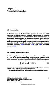
Fig. 6 Approximated and original curves of the five primary functions.
Proc. of SPIE Vol. 8768 87680F-6 Downloaded From: http://spiedigitallibrary.org/ on 02/05/2015 Terms of Use: http://spiedl.org/terms
Let N 20 , respectively,
T 30 , Nf is 3, 16, 8, 8 and 10 respectively, the approximated models are as the followings, yˆ x 4
(10)
yˆ 1.00 4.77 x 3.17 x 1.02 x 0.03x 2.48x sin 2 x 1.15x sin 2 x 1.70 x sin 2 x 1.22 x6 sin x 0.16 x6 sin 2 x 0.11x8 sin x 10 0.01x 5.23x sin x 10.11x2 sin x 10.19sin x 5.10sin 2x yˆ 1 0.88x 2.21x3 12.03x 4 3.54 x5 0.06 x8 3.54 x5 0.06 x8 0.02 x9 7.86 x3 sin x 2
4
6
8
2
3
4
yˆ x 0.17 x3 0.01x5
(11) (12) (13)
3 6 (14) yˆ 11.07 x 1.42 x3 0.06 x7 0.2 x8 0.06 x9 0.58x sin 2 x 0.37 x sin x Table 1 is comparison of integrals of 5 different functions based on EFN and other methods existing. Figure 6 is the approximated and original curves of the 5 primitive functions. The above two and formulas (11)-(14) show that EFN exactly approximates the original models; all expressed as linear combinations of generalized basis functions, and predicts the accurate domain of integration. The integrals by EFN are exactly the same with the accurate ones. Seen from (14), EFN can automatically achieve the model, which is coincident with Tailor expansion.
Example 2. Non-primary integral
1
e x dx 2
0
Let Nf 15 , T 30 , N 10 , the integral computed by EFN is 0.7468266418 with the approximated model followed, fˆ ( x) 1.00 3.03x3 14.20 x 4 56.28 x5 50.98 x 6 15.10 x 7 12.76 x sin( x) 2.80 x sin(4 x) 1.74 x 2 sin x 2.13 x3 sin(2 x)
(15)
4.65 x3 sin(4 x) 3.77 x 4 sin(3x) 3.11x5 sin(2 x) 5.74 x5 sin(3x) 0.01sin(3x) Table 2 .Integrals of
ex
2
based on efn and other methods existing
Accurate
EFN
MB-ES
DES
Simpso-n
Trapezo-id
Rectang-le
0.746824
0.7468266
0.74652
0.74683
0.74683
0.74621
0.77782
1.0
0.9
0.S
0.7
0.6
y 0.5 0.4 0.2
0.1
0.6
0.S
x
Original - Approximated
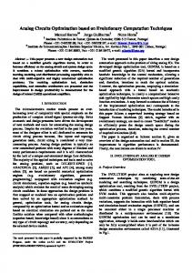
Fig. 7 The approximated and original curves of
ex
2
It can be seen from (15), Figure 7 and Table 2 that EFN not only can solve the primary ones but also the non-primary ones while the accuracy is also preserved. The integral by EFN is the most close to the accurate one compared with other methods existing.
Proc. of SPIE Vol. 8768 87680F-7 Downloaded From: http://spiedigitallibrary.org/ on 02/05/2015 Terms of Use: http://spiedl.org/terms
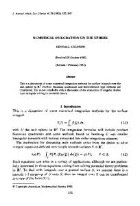
6. CONCLUSIONS Maybe more points are needed for accuracy compared with [5], especially in the case of highly oscillating function, but for those which have smooth curve, less is needed. Observing from the experiments, high accuracy is compensated for the more points. Genetic programming is effectively incorporated in the modelling of functional network, which overcomes the disadvantage of FN that, without background information of the problem, model and standard basis function family are hard to determine. At the same time, the subspace of the possible solution is narrowed by switching the object of encoding to generalized basis function. The advantage of GP is perfectly displayed that strong global search ability and the problem of "scale explosion" is overcome. Five experiments show that this algorithm is efficient for integration of all kinds of functions.
7. ACKNOWLEDGEMENTS This work supported by Grants 61165015 from National Science Foundation of China and by Grants 0991086 from Guangxi Science Foundation. Funded By Open Research Fund Program of Key Lab of Intelligent Perception and Image Understanding of Ministry of Education of China under Grant: IPIU012011001.
REFERENCES [1] [2] [3] [4]
[5] [6] [7] [8] [9] [10] [11] [12] [13] [14]
Kennedy J, Eberhart R C, Shi Y. Swarm Intelligence. San Francisco: Morgan Kaufman Publishers, 2001. Shi Y, Eberhart R C. A modified particle swarm optimizer. In: Proc. of the IEEE CEC. 1998: 69-73. Shi Y, Eberhart R C. Fuzzy adaptive particle swarm optimization. In: Proc. of the IEEE CEC. 2001: 101-106. Price K.V.. Differential evolution: A fast and simple numerical optimizer. Proceedings of the 1996 Biennial Conference of the North American Fuzzy Information Processing Society . Piscataway, NJ, USA: IEEE, 1996. 524527. Yang Qiwen, Cai Liang, Xue Yuncan. A survey of differential evolution algorithms. Pattern Recognition and Artificial Intelligence, 2008.8, 21(4): 506-513. He Q, Wang L. A hybrid particle swarm optimization with a feasibility-based rule for constrained optimization. Applied Mathematics and Computation, 2007, 186: 1407-1422. Rao S S. Engineering optimization (third ed). New York: Wiley, 1996. Deb K. Optimal design of a welded beam via genetic algorithms. AIAA Journal, 1991, 29: 2013-2015. Coello C A C. Use of a self-adaptive penalty approach for engineering optimization problems. Computers in Industry, 2000, 41: 113-127. Coello C A C, Montes E M. Constraint-handling in genetic algorithms through the use of dominance-based tournament selection. Advanced Engineering Informatics, 2002, 16: 193-203. He Q, Wang L. An effective co-evolutionary particle swarm optimization for constrained engineering design problems. Engineering Applications of Artificial Intelligence, 2007, 20: 89-99. Coello C A C, Becerra R L. Efficient evolutionary optimization through the use of a cultural algorithm. Engineering Optimization, 2004, 36: 219-236. Yongquan Zhou, Shengyu Pei. A hybrid Co-evolutionary particle swarm optimization algorithm for solving constrained engineering design problems. Journal of Computers, 2010, 5(6): 965-972. Arora J S. Introduction to Optimum Design. New York: McGraw-Hill, 1989.
Proc. of SPIE Vol. 8768 87680F-8 Downloaded From: http://spiedigitallibrary.org/ on 02/05/2015 Terms of Use: http://spiedl.org/terms