Numerical Simulation of Continuous Miner Rock ...

Numerical Simulation of Continuous Miner Rock Cutting Process

Bo Yu

Dissertation submitted to the College of Engineering and Mineral Resources at West Virginia University in partial fulfillment of the requirements for the degree of

Doctor of Philosophy In Mining Engineering

A. Wahab Khair, Ph.D., Chair Yi Luo, Ph.D. Syd S. Peng, Ph.D. Keith A. Heasley, Ph.D. Bruce Kang, Ph.D.

Morgantown, West Virginia 2005

Keywords: Numerical Simulation, Rock Mechanics, Rock Cutting, Continuous Miner Copyright 2005 Bo Yu

ABSTRACT Numerical Simulation of Continuous Miner Rock Cutting Process Bo Yu Usually, parametric analysis of the continuous miner cutting process is studied by experimental tests. In this dissertation, the need for numerical simulation of the continuous miner rock cutting process is established. In order to fulfill this need, four major numerical methods, namely the Finite Difference Method, the Finite Element Method, the Boundary Element Method, and the Discrete Element Method, are reviewed. The Finite Element Method is then chosen as the simulation tool because it is more advanced and versatile than the other methods. The rotation and advance of a continuous miner cutter head is simulated by the Finite Element Method with explicit time integration, while dynamic contact with an element erosion algorithm is utilized to model the impact between the bits and the rock elements. Two rock failure modes, shear failure and tensile failure, are implemented in the numerical model. By using the Automated Rotary Coal/Rock Cutting Simulator as the prototype, a numerical model of a continuous miner is developed and initially checked with experimental data. Then, several cutting parameters including: cutting speed, bit geometry, bit tip size, multiple bit interaction, and free face are studied using the thrust and cutting force calculated from the simulation. The specific work spent in each case is estimated by the thrust, cutting force, cutting time, and the volume of the removed rock. The grooves cut by the bits in the numerical model are used further to investigate the rock ridge failure mechanism. Shear failure is found to be the dominant failure mode for a continuous miner cutting an intact rock. In the conclusion the numerical modeling method is suggested as a valuable tool for parametric study of the rotary cutting process in the conclusion. And it can be advantageously used for continuous miner bit and drum design and prototype tests.

TABLE OF CONTENTS ABSTRACT....................................................................................................................... ii TABLE OF CONTENTS ................................................................................................ iii LIST OF FIGURES .......................................................................................................... v LIST OF TABLES .......................................................................................................... vii LIST OF SYMBOLS ..................................................................................................... viii ACKNOWLEDGEMENT............................................................................................. xiii Chapter 1 INTRODUCTION ......................................................................................... 1 1.1 Background ............................................................................................................. 1 1.2 Statement of the Problem........................................................................................ 2 1.3 Scope of Work ........................................................................................................ 6 Chapter 2 LITERATURE REVIEW ............................................................................. 7 2.1 Crack Modes in a Solid........................................................................................... 8 2.2 The Displacement Discontinuity Method and Its Application in Rock Cutting Simulation ............................................................................................................. 10 2.3 The Finite Element Method and Its Application in Rock Cutting Simulation ..... 13 2.4 The Finite Difference Method and Its Application in Tool-rock Interaction Simulation ............................................................................................................. 16 2.5 The Distinct Element Method and Its Application in Rock Cutting Simulation .. 19 2.6 New Techniques for Studying Crack Growth....................................................... 23 2.7 Summary ............................................................................................................... 24 Chapter 3 NUMERICAL TECHNIQUES APPLIED IN THE SIMULATION...... 25 3.1 The Governing Equations and Numerical Method Selection ............................... 25 3.2 The Finite Element Method with Explicit Time Integration ................................ 27 3.3 Interaction Algorithm with Erosion ...................................................................... 31 Chapter 4 COMPUTER SIMULATION OF ARCCS ................................................ 41 4.1 Model Setup .......................................................................................................... 41 4.2 Initial Results ........................................................................................................ 48 4.3 Summary ............................................................................................................... 55

iii

Chapter 5 EVALUATION OF CUTTING PARAMETERS ...................................... 66 5.1 The Effect of Cutting Speed in the Simulation..................................................... 66 5.2 The Effect of Bit Geometry .................................................................................. 71 5.3 Multiple Bit Interaction......................................................................................... 78 5.4 The Effect of Bit Tip Dimension on Impact Forces ............................................. 83 5.5 The effect of free faces ......................................................................................... 87 Chapter 6 ANALYSIS OF ROCK RIDGE BREAKAGE......................................... 94 6.1 Introduction........................................................................................................... 94 6.2 Numerical Simulation Results .............................................................................. 94 6.3 Discussion ............................................................................................................. 95 6.4 Mechanism of Rock Ridge Removal .................................................................... 98 6.5 Summary ............................................................................................................. 104 Chapter 7 SUMMARY AND CONCLUSIONS ........................................................ 105 7.1 Summary ............................................................................................................. 105 7.2 Final Conclusions................................................................................................ 107 7.3 Ideas for Additional Research............................................................................. 108 REFERENCE................................................................................................................ 109 APPENDIX: LIST OF LS-DYNA INPUT DECK ..................................................... 113

iv

LIST OF FIGURES Figure 1. 1 The automatic rock & coal cutting system ....................................................... 3 Figure 2. 1 Idealized model of the penetration of a wedge into rock ................................ 8 Figure 2. 2 The three modes of cracking ............................................................................ 9 Figure 2. 3 Illustrative meshes for fracture analysis with DDM...................................... 12 Figure 2. 4 Crack propagation simulated by Tan et al...................................................... 13 Figure 2. 5 The cracks illustrated explicitly in the FEM meshes (left), the smeared elements (right) ............................................................................................... 14 Figure 2. 6 The 2-D FE model in simulating rock ploughing........................................... 15 Figure 2. 7 The fracture propagation as the tool ploughs into the rock ............................ 16 Figure 2. 8 Normal indentation of a wedge into rock ....................................................... 18 Figure 2. 9 Particle interactions within cone crusher........................................................ 19 Figure 2. 10 Contact-bond Model in PFC2D................................................................... 21 Figure 2. 11 Rock specimen and tool for cutting simulation............................................ 22 Figure 2. 12 A moment in the rock cutting simulation .................................................... 22 Figure 3. 1 A cell structure .............................................................................................. 33 Figure 3. 2 Penetration check showing the pentahedral volumes which are computed. .. 34 Figure 3. 3 Assembly of normals from master elements to determine outside surfaces .. 35 Figure 3. 4 Diagram of slave node reposition................................................................... 38 Figure 4. 1 Bit block lacing pattern. ................................................................................. 42 Figure 4. 2 Cutting drum and rock in elements ................................................................ 43 Figure 4. 3 Various time stages in the cutting process I ................................................... 49 Figure 4. 4 Various time stages in the cutting process II.................................................. 50 Figure 4. 5 Cutting grooves comparison.......................................................................... 51 Figure 4. 6 Diagram of contact forces .............................................................................. 53 Figure 4. 7 The initial angle of each bit on the drum........................................................ 53 Figure 4. 8 The thrust and cutting forces of bit 1.............................................................. 56 Figure 4. 9 The thrust and cutting force of bit 2 ............................................................... 57 Figure 4. 10 The thrust and cutting force of bit 3 ............................................................. 58 Figure 4. 11 The thrust and cutting force of bit 4 ............................................................. 59 Figure 4. 12 The thrust and cutting force of bit 5 ............................................................. 60 Figure 4. 13 The thrust and cutting force of bit 6 ............................................................. 61 Figure 4. 14 The thrust and cutting force of bit 7 ............................................................. 62 Figure 4. 15 The thrust and cutting force of bit 8 ............................................................. 63 Figure 4. 16 The thrust and cutting force of bit 9 ............................................................. 64 Figure 4. 17 Total thrust and cutting force of the drum.................................................... 65

v

Figure 5. 1 Total thrust and total cutting force of the drum cutting rock with a rotation rate of 5,250 rad/sec and an advancing rate of 200 in/sec................. 69 Figure 5. 2 Total thrust and total cutting force of the drum cutting rock with a rotation rate of 2,625 rad/sec and an advancing rate of 200 in/sec................. 70 Figure 5. 3 Bit models used in the simulation .................................................................. 72 Figure 5. 4 Bit tip and bit body thrust comparison for bit model 1 .................................. 72 Figure 5. 5 Bit tip and bit body cutting force comparison for bit model 1 ....................... 73 Figure 5. 6 Bit tip and bit body thrust comparison for bit model 2 .................................. 74 Figure 5. 7 Bit tip and bit body cutting force comparison for bit model 2 ....................... 75 Figure 5. 8 Cutting grooves comparison........................................................................... 78 Figure 5. 9 The thrusts of bit 6 in single bit cutting and multiple bit cutting ................... 79 Figure 5. 10 The cutting forces of bit 6 in single bit cutting and multiple bit cutting ............................................................................................................. 80 Figure 5. 11 Cutting groove comparison between double bit penetration and single bit penetration....................................................................................... 80 Figure 5. 12 Cutting groove comparison between double big bit cutting and single big bit cutting........................................................................................ 81 Figure 5. 13 The thrusts of big bit 6 in two conditions and the difference....................... 82 Figure 5. 14 The cutting forces of big bit 6 in two conditions and the difference............ 83 Figure 5. 15 Total thrust and total cutting force of the drum installed with 9 big bits cutting rock with a rotation rate of 5,250 rad/sec and an advancing rate of 200 in/sec. .......................................................................... 86 Figure 5. 16 Total thrust and total cutting force of the drum installed with 4 big bits cutting rock with a rotation rate of 5,250 rad/sec and an advancing rate of 200 in/sec. .......................................................................... 87 Figure 5. 17 Grooves cut by the drum with two pre-cutters at each side ......................... 88 Figure 5. 18 Total thrust and total cutting force of the drum with two pre-cutters cutting rock ..................................................................................................... 90 Figure 5. 19 The thrusts and cutting forces of bit 4 acted as a pre-cutter and acted as a normal cutter................................................................................... 91 Figure 5. 20 The thrusts and cutting forces of bit 1 beside a pre-cutter and beside a normal cutter. .................................................................................... 92 Figure 5. 21 The thrusts and cutting forces of bit 2 in cutting processes with a pre-cutter and without a pre-cutter.................................................................. 93 Figure 6. 1 Cutting grooves of bit 1 in three numerical tests............................................ 95 Figure 6. 2 A projectile penetrates a rock plate ................................................................ 97 Figure 6. 3 The projectile penetrated through the rock plate............................................ 97 Figure 6. 4 Nodal forces in a rock element due to bit penetration.................................... 99 Figure 6. 5 E and µ effect on the ridge removal ............................................................. 100 Figure 6. 6 Sumping and cutting action in high E and µ value rock cutting .................. 100 Figure 6. 7 Multiple bit interaction ................................................................................. 102 Figure 6. 8 Cutting depth effect on the ridge removal.................................................... 102 Figure 6. 9 Drum advance rate effect on the ridge removal ........................................... 103 Figure 6. 10 The rock compressive strength effect on ridge removal ............................ 103

vi

LIST OF TABLES Table 4.1 Parts for contact definition ………………………………………………… 44 Table 4.2 The mechanical properties of materials ……………………………………

45

Table 5.1 Average values of the total thrust and the cutting force for situation 1 to 3 . 68 Table 5.2 The thrusts and cutting forces and their specific energy …………………..

vii

77

LIST OF SYMBOLS E

Young’s modulus

µ

Poisson’s ratio

Fc

cutting force

Wc

work done by cutting force

Ft

thrust force

Wt

work done by thrust

L

total cutting trace length

d

final depth of cut

W

work done by thrust and cutting force

SE

specific energy

Vc

volume of cut off material

pr

depth of penetration per revolution

β

half of tip angle

σ ij

Cauchy stresses

σ ij'

deviatoric stress components

p

pressure

ρ

density of material

I1

first invariant of the stress tensor

σt

tensile strength of the rock

σc

compressive strength of the rock

σ1

maximum principal stress

viii

GI(θ)

mode I strain energy release rate

GII(θ) mode II strain energy release rate GIC

mode I critical energy release rate

GIIC

mode II critical energy release rate

ui

displacement vectors on the boundary in Equation 2.2.4

ti

traction vectors on the boundary in Equation 2.2.4

∆ ui

displacement jumps across two opposite surface of a fracture

∆ ti

traction jumps across two opposite surface of a fracture

u*ij

fundamental solutions of displacement

t *ij

fundamental solutions of traction

*

u ij *

fundamental solutions of displacement

t ij

fundamental solutions of traction

cij

free terms in Equation 2.2.4 and 2.2.5

φI

interpolant

uI

value of a neighborhood node which locates in the circle of influence in Equation 2.6.1

H(x)

heaviside function

bI

coefficient in Equation 2.6.1

FL(x) displacement fields in front of crack tip Ω

domain

Ωe

element domain

Г

boundary of the domain

ix

Γt i

union of traction boundaries

Γint

union of all surfaces on which the stresses are discontinuous

b

body force per unit mass

t

traction per unit area

v

velocity vector of a particle

d/dt

material derivative

δv i

test function

δP int

total virtual internal power

δP ext

virtual external power

δP kin

virtual inertial power

N I ( X) shape functions uI

nodal displacements

I

nodal number

v (X, t ) nodal velocity X

nodal coordinates

t

time

u& I

nodal velocity

fiIint

internal nodal forces

f iIext

external nodal forces

fiIkin

inertial (or kinetic) nodal forces

a

column matrices of the unconstrained accelerations

f

column matrices of the unconstrained nodal forces

x

M

mass matrix for the unconstrained degrees of freedom

&& u

accelerations

tE

simulation time

∆t n

time step

∆t crit

critical time step

n TS

number of time steps

gI

generalized representation of the displacement boundary conditions and other constraints on the model

ωmax

maximum frequency of a lineared system

le

characteristic length of an element

ce

current wave speed in an element

α

reduction factor in Equation 3.2.18

α

rotation angle of the bit in Equation 4.2.1

R e2

radius of an element

n

vector normal to an element side

n

average normal of a master element

×

vector cross-product in Equation 3.3.5 vector length

η

undetermined parameter η > 0 in Equation 3.3.7

x0

initial coordinates of a slave node in Equation 3.37

xn

current coordinates of a slave node in Equation 3.37

xi

xf

final coordinates of a slave node

ξI

undetermined parameters in Equation 3.3.9

∆r

change of displacement for a slave node

∆v

change in velocity for a slave node

v new

new velocity of a slave node

v old

old velocity of a slave node

m

mass of a slave node

fd

viscous damper force

dc

damping constant

A

area of the element face on the non-reflecting boundaries

X

x direction contact force between the bit and the rock

Y

y direction contact force between the bit and the rock

R

resultant force of X and Y

n

revolution number of the drum

r

cutting radius of a bit

θ

initial angle of a bit

xii

ACKNOWLEDGEMENT I would like to thank Dr. A. W. Khair for the opportunity to do this research and for his invaluable instructions and kind encouragement throughout my graduate study. I would also like to convey my thanks and appreciation to the other committee members, Dr. Syd S. Peng, Dr. Yi Luo, Dr. Keith A. Heasley, Dr. Bruce Kang, and Dr. Venkata Babu Achanti, for their constructive criticisms and concrete suggestions at several stages of this work. I am thankful to the Coal and Energy Research Bureau (CERB), State of West Virginia, for their financial support during the course of this research work. Special thanks goes to my parents, my wife, Hua, and my two daughters, Anqi and Nova, for their love and encouragement.

xiii

Chapter 1 INTRODUCTION 1.1 Background The continuous miner has been utilized since about 1945 (Kegel, 1973). It uses a cylinder-shaped cutter drum, approximately 40 inches in diameter and 10 feet long. The rotating drum with conical bits laced on it can be fed or sumped into the face to cut the coal. This continuous mechanical excavation machine has many advantages over the conventional drill & blast technique. These include (Cigla and Ozdemir, 2000):

•

High productivity/advance rates

•

Improved safety

•

Minimal ground disturbance

•

Reduced support requirement

•

Elimination of blast vibrations

•

Reduced ventilation requirements

•

A uniform size of rock fragmentations Under the requirements of improving productivity and reducing cost per ton of coal,

manufacturers are supplying heavier, more powerful continuous miners. For example, DBT’s 40M series continuous miners weigh 225,000 pounds and have 700 horsepower for the cutting head (DBT’s webpage). The latest continuous miners feature much higher cutting forces and greater penetration speed, and become more capital intensive and site specific today. Therefore its performance under specific conditions must be understood in order to most efficiently utilize these machines.

1

1.2 Statement of the Problem The cutting parameters influencing continuous miner performance include rock properties, cutting speed, bit geometry, bit tip size, multiple bit interaction, free face formation, etc. Efficient utilization of continuous miners depends on fully understanding the parameters described above. Some experimental studies have addressed the effects of the above variables on the efficiency of the continuous miner. A linear cutting test program was conducted to simulate rotary cutting of continuous miner (Asbury, Cigla and Balci, 2002). In this test program, the thrust required to penetrate rock by a continuous miner was derived from the normal force. The cutting drum torque requirement by a continuous miner was represented by a function of the thrust. It was assumed that the ratio of the drag force over the normal force can provide a measure of the direction that the bit is being loaded in rotary cutting. Whenever full scale linear cutting results were not available, the cutting forces ( Fc ) were estimated by Evans’ formula (1984) where 2

16σ 2t p r Fc = cos(β) 2 σ c

(1.2.1)

where: Fc is the cutting force (kN), pr is depth of penetration per revolution (mm), β is half of tip angle (degree), σ t is tensile strength of the rock (MPa), σc is compressive strength of the rock (MPa).

2

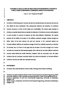
An Automated Rotary Coal/rock Cutting Simulator (ARCCS) was developed to evaluate the cutting parameters influence on the cutting results (Khair, 1984). The ARCCS, shown in Figure 1.3a, included a main frame, a confining chamber, and a cutting drum. Figure 1.3b shows the monitoring equipments which was used to monitor the penetration and cutting pressure of the frame, cutting depth, advance rate, and the count number of acoustic emission.

A

B

Figure 1. 1 The automatic rock & coal cutting system

A series of experiments have been conducted on the ARCCS since it was built. Devilder (1986) correlated the fragment size distribution and the characteristics of the fracture surface in coal cutting under various testing conditions. The correlation was based on a series of forty-three tests conducted in the laboratory using the ARCCS. It was concluded that the parameters: bit type, bit spacing, depth of cut, in-situ stresses, and cleat orientation have an apparent contribution to the fragment size distribution and the fracture surface. The two exceptions were bit attack angle and cutting head velocity. Using three bits simultaneously mounted on the cutting drum of the ARCCS, Achanti (1998) used an orthogonal fractional factorial experimental plan to investigate 3

the nature of ridge failure and the effects of bit spacing, cutting depth, cutting head rotational speed, and bit tip angle on respirable dust generation. It was found that a clean cutting surface results due to larger bit tip size at greater cutting depths. Addala (2000) investigated the relationship between cutting parameters (cutting force, penetration force, specific energy, and specific respirable dust) and the bit geometry parameters (angle of the bit tip, and bit tip size) in order to reduce the amount of specific dust generated and the specific energy consumed in rotary cutting. The experimental values of penetration force and cutting force showed that as the tip angle increases the amount of forces required to cut the rock increases, But when there is a free face available adjacent to a cut it requires less force to cut the rock. The results also showed that the specific energy reduces as the bit size increases, because a larger bit produces more rock product and therefore the specific energy is reduced. Experiments were carried out by Venkataraman (2003) to study the effect of rate of advance of the ARCCS on the rock fragmentation. The rock material was Indiana limestone. Since it was too strong for the ARCCS to effectively cut, the maximum depth of sumping was used to evaluate the cutting efficiency. It was found that optimum values of free face and bit spacing together increase the efficiency of the cutting system. As the depth of free face increases, the depth of subsequent cuts increase. Qayyum (2003) evaluated the effects of bit geometry in multiple bits-rock interaction, utilizing the ARCCS and synthetic rock. During the experiments, 9 bits were mounted on the drum and 5 different kinds of bits were tested. A similar conclusion was drawn as Addala (2000). It was found that a larger bit tip results in a higher resultant

4

force. However the trend in the specific energy was opposite to the trend in the resultant forces. From the previous experimental studies on the LCM and ARCCS, it can be concluded that experimental study is a direct method to investigate the effects of the cutting parameters (i.e. bit geometry, bit spacing, advance rate, depth of cut, etc.) on the cutting results (cutting force, penetration force, specific energy, etc.). However, for the LCM the penetration depth was always constant so that it is not suitable to derive rotary cutting forces from the drag and normal force of the LCM, since in a rotary cutting situation the depth of cut of a bit varies from zero at the beginning to the maximum depth at the middle of the cutting trace, the depth of cut then falls back to zero when the bit looses contact with the rock/coal. Limited by its power, the ARCCS is hard to simulate the current continuous miners’ full bit penetration depth. In both cases the property inconsistence of test materials can have large influence on the test results so that a large number of tests would have to be conducted in order to obtain an average level of the machine performance. It is time consuming and costly to prepare specimens and conduct tests. Some experimental conclusions were based on a very limited number of tests, which had no statistical significance. Therefore, a numerical model, which can accurately calculate the cutting forces and specific energy in different cutting conditions, would be extremely useful. Recent developments in numerical simulation technologies have made it possible to model a continuous miner cutting process. Four major numerical methods, namely, the Finite Element Method, the Finite Difference Method, the Discrete Element Method, and the Boundary Element Method and their applications in rock cutting simulation will be

5

discussed in Chapter 2. Based on the continuous miner model and rock model built in the computer, a series of numerical experiments will be conducted. This would overcome the shortcomings of the experimental tests by accurately simulating the rotary cutting situation and keeping the rock properties constant when investigating other variables.

1.3 Scope of Work The objective of this work is to simulate the continuous miner rotary cutting process using a numerical model. The numerical model will not only be able to calculate the cutting forces but will also be able to calculate the volume of material removed. The intention is to implement a dynamic contact algorithm into the model and simulate the excavated material by eroding failed elements. The ARCCS will be chosen as a prototype for the numerical model. The simulation results will be calibrated and verified initially by cutting results of tests on the ARCCS. Then, the cutting parameters such as: rock properties, cutting speed, bit geometry, bit tip size, multiple bit interaction, and free face, etc. will be evaluated through numerical experiments. To further broaden the scope, it is proposed to include the capability of rock failure mode recognition in the model. A dichotomy exists between the two theories of rock failure – tensile and shear. By turning off one of the criteria, the rock failure mode in rotary cutting can be evaluated. The rock material will be modeled as elastic material before failure. This will greatly simplify the computation time of the model. The rock material will be defined by strengths, Young’s modulus, and Poisson’s ratio.

6

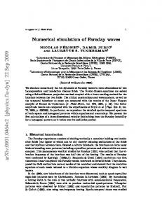
Chapter 2 LITERATURE REVIEW The basic mechanism of continuous miner rock cutting is tool (i.e. bit) – rock interaction. Tool-rock interaction has been a subject of study since the 1950’s. It is known now that the rock fragmentation process due to tool indentation generally includes the following stages (shown in Figure 2.1): initiation of the stress field, formation of an inelastic deformation zone or a crushed zone, chipping and crater deformation of the surface, and formation of subsurface cracks (Mishnaevsky, 1998). However, rock cutting, rock drilling and ploughing processes are much more complicated than simple indentation. Among the aspects of cutting that are different from indentation, one can mention non-vertical loading direction, non-axisymmetric shape of tool, interaction of existed crack system with the free surface, and continuity of the process of chip removal. All these factors significantly change the mechanism of rock fragmentation. Because experimental investigations of the rock cutting process are most time consuming and it is difficult to directly observe the material removal process, numerical tools have been developed to elucidate rock-tool interaction during rock cutting. Two different approaches have been used to model rock fragmentation depending on how the damage is represented: either by explicitly modeling of the rock fracture process or by constitutive relations developed in continuum mechanics. The numerical methods most widely used for analysis of tool-rock interaction are the Finite Difference Method (FDM), Finite Element Method (FEM), Boundary Element Method (BEM) and Discrete Element Method (DEM).

7

Figure 2. 1 Idealized model of the penetration of a wedge into rock (After Paul and Sikarskie, 1965) In this review, the numerical studies on rock indentation and rock cutting will be summarized. The rock failure modes and failure criteria will be discussed first. Then the applications of four numerical methods, namely the DDM, the FEM, the FDM, and the DEM on rock cutting simulation will be reviewed. New techniques for simulation of crack growth will also be presented. The discussions on these methods are in the last section.

2.1 Crack Modes in a Solid According to conventional fracture mechanism theory, a crack in a solid can be stressed in three different modes, as illustrated in Figure 2.2. Normal stresses give rise to the “open mode” denoted as mode I. The displacements of the crack surfaces are perpendicular to the plane of the crack. In-plane shear results in mode II or “sliding modes”: the displacement of the crack surfaces is in the plane of the crack and perpendicular to the leading edge of the crack. The “tearing mode” or mode III is caused

8

by out-of-plane shear. Crack surface displacements are in the plane of the crack and parallel to the leading edge of the crack. The superposition of the three modes describes the general case of cracking (Broek, 1982). It is believed that in the rock cutting process, the crack can propagate in these three modes (Shen, 1993, Wang, 1995).

Figure 2. 2 The three modes of cracking

Two fracture criteria, based on stress and energy respectively, have been applied to explain the propagation of a brittle fracture. Their major features are listed as follows: (1) Stress criterion •

The propagation of a crack requires that the local tensile stress developed around the tip of the crack must be larger than the uniaxial tensile strength of the material.

•

The direction of possible crack propagation is perpendicular to the direction of the maximum tensile stress developed around the crack.

9

(2) Energy release rate criterion The energy release rate criterion is based on the fact that the formation of a crack requires a certain amount of energy. Crack extension can occur when the energy release rate (G) is equal to the energy required for crack growth, which is called crack resistance (Gc). Shen and Stephansson (1993) proposed the F-criterion based on the energy release criterion to simulate the mixed-mode (mode I and mode II) fracture propagation. The principle of the F-criterion can be stated as follows: •

In an arbitrary direction (θ) at a fracture tip, there exists a F-value, with F(θ) =

G I (θ) G II (θ) + G IC G IIC

(2.1.1)

where GI(θ) and GII(θ) are the mode I and II strain energy release rates, GIC and GIIC are their critical energy release rates respectively. •

The possible direction of propagation of the fracture tip (θ0) is the direction for which the F-value reaches its maximum.

F(θ) θ = θ = max

(2.1.2)

0

•

When the maximum F-value is equal to or larger than 1.0, the fracture tip will propagate, i.e. F(θ) θ = θ ≥ 1.0

(2.1.3)

0

2.2 The Displacement Discontinuity Method and Its Application in Rock Cutting Simulation The Displacement Discontinuity Method (DDM) is an indirect Boundary Element Method (BEM) which was developed by Crouch and Starfield (1983). By using the following techniques: a weighted residual formulation, Green's third identity, Betti's

10

reciprocal theorem or some other methods, the DDM transforms Partial Differential Equations (PDEs) to an equivalent integral equation, and then converts to a form that involves only surface integrals, i.e., over the boundary (Hunter, 2003, Wen, 1996, Jing, 2003). The DDM has an advantage for the simulation of crack growth because the fractures can be represented by single fracture elements without the need for separate representation of their two opposite surface. Denote Гc as the path of the fracture which is in the domain Ω whose boundary is denoted by Г (shown in Figure 2.3). The basic integral equation of the DDM can be written as:

u i = c ij ∆u j + ∫ u *ij ∆u j dΓ + ∫ u ij ∆u j dΓ

(2.2.4)

t i = c ij ∆u j + ∫ t *ij ∆u j dΓ + ∫ t ij ∆u j dΓ

(2.2.5)

*

Γ

Γc

*

Γ

Γc

where ui and ti are the displacement and traction vectors on the boundary Г, ∆ ui and ∆ ti are the displacement and traction jumps across the two opposite surface of the fractures, *

*

u*ij and t *ij , u ij and t ij are fundamental solutions of displacement and traction, cij is called

the free terms, see Wen (1996) and Jing (2003) for details. In order to solve integral equations (2.2.4) and (2.2.5), the boundary and fracture are first discretized into elements. Then, the displacement discontinuities at the fracture nodes are calculated. After stress intensity factors for different fracture modes are determined, the fracture growth will be calculated based on fracture propagation criteria.

11

Figure 2. 3 Illustrative meshes for fracture analysis with DDM (After Jing, 2003) A rock indentation model was developed by Tan et al. (1996), in which the Fcriterion was incorporated into a DDM code. The initial cracks were introduced along the crushed zone boundary. The fracture growth patterns of simulated indentation cracks in granite are shown in Figure 2.4. In this DDM model the crack coalescences with indentations of two hemispherical indenters in granite were tested. It was found that cracks only at specific locations and orientations can generate coalescence; others will either have no development or miss each other. The advantages of the DDM can be summarized as follows: •

The DDM can model the crack growth in rock under indentation.

•

Compared with the finite element methods and the finite difference methods, the DDM generates much simpler mesh.

12

However only the above application on modeling rock indentation has been studied to date.

S=5a, coalescence

a) Crack pattern of hemispherical indentation (F=60kN) S=6a, no coalescence

b) Crack pattern of truncated indentation (F=90kN)

Figure 2. 4 Crack propagation simulated by Tan et al.

2.3 The Finite Element Method and Its Application in Rock Cutting Simulation The Finite Element Method (FEM) has been successfully applied to a wide class of partial differential equations. Strang and Fix (1988) contributed the success of the FEM to its choice of piecewise polynomials as trial function. Piecewise polynomials were becoming preeminent in the mathematical theory of approximation of functions at the time when the FEM was created. So, the FEM has sound mathematical foundations. It is considered as the right idea at the right time. When simulating the process of fracture growth, the FEM is handicapped by the requirement of small element size, continuous re-meshing with fracture growth, and conformable fracture path and element edges. Although numerical difficulties exist, the finite element method has been widely used for studying fracture problems. A special finite element technique called the ‘smeared crack’ approach has been used in tool-rock

13

interaction problems. In this technique, the stress in each element is monitored. The failed element remains a continuum but loses its load carrying capacity (stiffness and/or strength) in certain directions. The cracks are not represented explicitly, but modeled as ‘smeared cracks’ by modifying the material constitutive relations in a suitable way (shown as Figure 2.5). The methodology is relatively simple to implement, and doesn’t need mesh refinement.

Figure 2. 5 The cracks illustrated explicitly in the FEM meshes (left), the smeared elements (right) This method has been used by Wang (1975), Zeuch et al.(1983), Korinets and Chen (1996), Tang (1997), Kou et al. (1999) and Liu (2002) to simulate fracture propagation during rock indentation or rock cutting. Generally these models used a stress based criterion to form cracks normal to the maximum principal stress (tensile stresses taken as positive) at the element integration points. Failure occurs if the maximum tensile stress exceeds the specified fracture strength. In compression, the models utilized a MohrCoulomb failure criterion to form shear cracks at the element integration points. After the cracks have formed, the strains normal to both the tensile and shear cracks are monitored in subsequent time/load steps to determine if the cracks are open or closed. If a crack is open, the normal and shear stresses on the crack face are set equal to zero for a tensile crack. Wang (1975) also used the ‘stress transfer’ method suggested by Zienkiewicz 14

(1968) to convert excessive stresses that an element cannot bear to nodal loads and reapplies these nodal loads to the element nodes and thereby to the system. If a crack is closed, a compressive normal stress can be carried, but the shear stress is limited to a value described by the Coulomb friction model. Figure 2.6 and Figure 2.7 shows the simulation of fracture propagation and coalescence in the rock ploughing process using the smeared crack approach by Liu (2002). The rock was simulated as a heterogeneous material by assigning different material properties to element zones. The smeared crack approach has several disadvantages which has limited its application. First, the results of crack propagation simulations are highly sensitive to the mesh size used. But if elements in the region of the expected crack path become too small, there may arise a lack of convergence in the dynamic FEM. Second, since the stresses and strains are calculated at the integration points of the elements, these stresses or strains are smaller than those at the crack tip. Therefore, the overall displacements in the model may be accurate, but stresses and strain energies calculated with finite elements will be inaccurate in the crack region.

Figure 2. 6 The 2-D FE model in simulating rock ploughing

15

Figure 2. 7 The fracture propagation as the tool ploughs into the rock

2.4 The Finite Difference Method and Its Application in Tool-rock Interaction Simulation In the finite difference method, every derivative in the set of governing equations is replaced directly by an algebraic expression written in terms of the field variables (e.g., stress or displacement) at discrete points in space (Itasca, 2001). Without iterative solutions of the global matrix equation systems as in the FEM, the FDM has an advantage in simulating complex constitutive material behavior, such as plasticity and damage.

16

However, explicit representation of fractures is not easy in the FDM because it requires continuity of the functions between the neighboring grid points. The FDM can still use the smeared crack approach to catch material failure or damage propagation at the grid points or cell centers without creating fracture surfaces specifically in the models. At present, the most well known finite difference code used in rock engineering problems is perhaps the FLAC code group. It uses the finite difference approach combined with the Finite Volume Method (FVM) and can treat arbitrary boundary conditions and material heterogeneity. Damjanac and Detournay (1995) used a finite difference code (FLAC) to simulate the problem of wedge indentation into an elasto-plastic half-plane (As shown in figure 2.8). Their study focused on the initial regime of the indentation process (prior to the initiation of a tensile fracture). It was found that the indentation process is predominantly controlled by a single number, which is a function of: the wedge angle, the unconfined compressive strength of the rock, and its elastic modulus. Huang et al. (1998) used FLAC to investigate the influence of the lateral confining stress of the rock on the initiation of the tensile fractures. The results of her numerical study suggested that the initiation of tensile cracks is to a great extent controlled by lateral confinement. It was presumed that the tensile crack would take place at the point of maximum tensile stress on the boundary of the plastic zone (i.e. crushed zone). Lateral instead of vertical cracks would first be initiated on the boundary of the crushed zone with increasing confinement.

17

Figure 2. 8 Normal indentation of a wedge into rock (After Damjanac and Detournay, 1995)

An extraordinary application of FLAC can be found in Clark’s study (1999) in which the rock crushing process inside the crusher was simulated (shown in Figure 2.9). One hundred discrete particles of different sizes created in the FLAC grid were gravity fed into the crusher. To ensure interaction between all particles and their interaction with the crusher liners, 7120 interfaces had to be declared. Particle fracture was represented by nulling zones which became tensile. The model ran continuously over a period of months. FLAC was used here as a distinct element code.

18

Figure 2. 9 Particle interactions within cone crusher (After Clark 1999)

2.5 The Distinct Element Method and Its Application in Rock Cutting Simulation Distinct Element Methods (DEM) are numerical procedures for simulating the complete behavior of systems of discrete, interacting bodies. The theoretical foundation of the method is the formulation and solution of equations of motion of rigid and/or deformable bodies using implicit and explicit formulations. The most well-known codes for modeling granular materials are the Particle Flow Codes (PFC) for both two-dimensional and three-dimensional problems. The code

19

models solids as a collection of distinct and arbitrarily sized circular particles. The overall constitutive behavior of a material is simulated by associating a simple constitutive model with each contact. The three constitutive models governing the contacts between particles are: a stiffness model, a slip model, and a bonding model. The stiffness model provides an elastic relation between the contact force and relative displacement. The slip model enforces a relation between shear and normal contact forces such that the two contacting balls may slip relative to one another. The bonding model serves to limit the total normal and shear forces that the contact can carry by enforcing bond-strength limits. Huang et al., (1999) and Lei and Kaitkay (2003) performed numerical simulation of rock cutting using PFC2D. Both of them used the contact-bond model to simulate the constitutive behavior of rock material. A contact bond can be envisioned as a pair of elastic springs (or a point of glue) with constant normal and shear stiffness acting at the contact point (shown in Figure 2.10). These two springs have specified shear and tensile normal strengths. The mechanism of the contact-bond model is in many ways similar to the smeared crack approach in FEM: if the magnitude of the tensile normal contact force equals or exceeds the normal contact bond strength, the bond breaks, and then, both the normal and shear contact forces are set to zero. If the magnitude of the shear contact force equals or exceeds the shear contact bond strength, the bond breaks, but the contact forces are not altered, provided that the shear force does not exceed the fiction limit, and provided that the normal force is compressive. After the contact bond is broken, the slip model is active.

20

Illustration of bond contact

Constitutive behavior for contact occurring at a point Figure 2. 10 Contact-bond Model in PFC2D (After PFC2D 3.0 Manual) Figure 2.11 shows the PFC model for a rock cutting simulation. The rock is simulated as different sizes of discs bonded together. The cutting tool was modeled as a rigid edge. The cutting forces can be predicted and the failure modes of the rock can also be detected. The specimen damage plot shown in Figure 2.12 provides cracking information.

21

Figure 2. 11 Rock specimen and tool for cutting simulation (After Lei, 2003)

Figure 2. 12 A moment in the rock cutting simulation The major advantage of the DEM approach is that a physical fracture or crack can be formed and propagated explicitly during calculation. The disadvantage of this method is that the tools can only be treated as rigid and can only move at a given speed which is independent of any resistance from the particles. This limits its ability to study the toolrock interaction.

22

2.6 New Techniques for Studying Crack Growth In the past decade there were mainly two new techniques developed to simulate fracture propagation explicitly: one is the Element-Free Galerkin Method (EFG), the other is the Enriched Finite Element Method (XFEM). It is believed that these two methods will play a significant role in the next generation of computer simulation of fractures. These two methods are introduced briefly below: (1) Element-Free Galerkin Method The Element Free Galerkin Methods have been an active research area in recent years. The method is completely element free. It is only necessary to construct an array of nodes in the domain under consideration. A user could simply drop a large number of points into the portion of a component where he would like more accuracy. In this method, moving least-squares interpolants are used to construct the trial and test functions for the variational principle (weak form). The interpolants are polynomials which are fit to the nodal values by a least-squares approximation. Dolbow et al. (1999) used the following interpolant to simulate the crack surfaces, u h ( x ) = ∑ φI [u I + H( x )b I + ∑ c IJL FL ( x )] I

(2.6.1)

J

where φI is the interpolant, u I is the value of a neighborhood node which locates in the circle of influence, H(x) is the heaviside function, bI is the coefficient which can be determined by minimizing the local interpolation error. FL(x) are the displacement fields in front of crack tip. The H( x )b I + ∑ c IJL FL ( x ) term is called the enrichment functions. J

These functions allow for the proper jump in field variables along the crack.

23

This method can easily handle damage of the components, such as fracture, which should prove very useful in modeling of material fracture. (2) Enriched Finite Element Method The enriched Finite Element Method came naturally when the interpolant φ I in equation (2.6.1) is substituted by the standard finite element shape functions. To contrast this method with the Element Free Galerkin Method, it is truly a finite element method and can exploit the large body of finite element technology and software. The crack is represented as a discontinuity in the displacements within the element. This method can simulate crack growth without continuous remeshing.

2.7 Summary 1. Simulation of fracture propagation and the dynamic contact between tool and rock are two necessary aspects in modeling tool-rock interaction. These two areas are also among the most difficult and challenging problems in numerical modeling. 2. Among the numerical methods mentioned above: •

The DDM is efficient for simulating fracture problems.

•

The DEM can handle fracture propagation and dynamic contact “naturally”.

•

The FDM and the FEM are much more developed and versatile than the others.

3. Numerical simulations of tool-rock interaction are limited by the shortcomings of the available numerical techniques.

24

Chapter 3 NUMERICAL TECHNIQUES APPLIED IN THE SIMULATION During the continuous miner rock cutting process, the penetration and cutting of the bits cause the rock broken. If the spatial distribution of the displacement over the rock at any given time is known, then the stress state of a point in the rock can be calculated by the displacement strain relationship and the constitutive equations. Therefore, the displacement or the velocity of a point in the rock mass can be treated as a basic unknown.

3.1 The Governing Equations and Numerical Method Selection Provided Newton’s Third Law of Action and Reaction governs the internal particles’ movement, then the time rate of change of the total momentum of a given set of particles equals the vector sum of all the external forces acting on the particles of the set. This is the basic postulate in the derivation of the governing equations in a continuous medium (Malvern, 1969). Consider a given mass of the medium, instantaneously occupying a domain Ω bounded by surface Γ and acted upon by external surface traction t per unit area and body forces b per unit mass. The rate of change of the total momentum of the given mass is (d / dt ) ∫ ρvdΩ , where d/dt denotes the material derivative of the integral, ρ is the density of material, v is the velocity vector of a particle in the volume. Then, the momentum balance expressed by the postulate is

∫ tdΓ + ∫ Γ

Ω

ρbdΩ =

d ρvdΩ dt ∫ Ω

(3.1.1)

in rectangular coordinates

25

∫

Γ

t i dΓ + ∫ ρb i dΩ = Ω

d ρv i dΩ dt ∫ Ω

(3.1.2)

Substitute the traction boundary conditions:

t i = σ ji n j on Γt i

(3.1.3)

where Γt i is the union of traction boundaries and transform the surface integral by using the divergence theorem to obtain

∫

Ω

(

∂σ ji ∂x j

+ ρb i )dΩ = ∫ ρv& i dΩ

(3.1.4)

Ω

Hence the momentum balance takes the form

∫

Ω

(

∂σ ji ∂x j

+ ρb i − ρv& i )dΩ = 0

(3.1.5)

for an arbitrary domain Ω , at each point we have ∂σ ji ∂x j

+ ρb i = ρv& i

(3.1.6)

This balance of momentum is the basic governing equations in our problem. As we discussed in Chapter 2, there are several broad numerical techniques available. The most well-known commercial software to solve Equation (3.1.6) is LSDYNA3D. LS-DYNA3D is an explicit finite element code for analyzing the dynamic response of three-dimensional solids and structures. The element formulations available include one-dimensional truss and beam elements, two-dimensional quadrilateral and triangular shell elements, two-dimensional delamination and cohesive interface elements, and three-dimensional continuum elements. Many material models are available to represent a wide range of material behavior, including elasticity, plasticity, composites, thermal effects, and rate dependence (DYNA3D User Manual, 1999).

26

In addition, LS-DYNA3D has a sophisticated contact interface capability to handle arbitrary mechanical interactions between independent bodies or between two portions of one body. In order to treat the dynamic contact between the bit tip and rock, an algorithm of contact with erosion developed by Belytschko and Lin (1985) was chosen. The basic purpose of this algorithm is to treat the interaction of two bodies with eroding elements. Eroding elements are elements which are destroyed during the course of the computation because of very high strains. They are used to represent rock material removed by bits in this dissertation. In this chapter, the finite element method with explicit time integration will be discussed briefly, and the impact and penetration algorithm will also be described. The complete algorithm steps will be summarized in the end.

3.2 The Finite Element Method with Explicit Time Integration 3.2.1 The Weak Form of the Governing Equation In the finite element method, we seek a solution to the momentum equation (3.1.6) which satisfies the traction boundary conditions (3.1.3) and the traction continuity conditions

[ n jσ ji ] = 0 on Γint

(3.2.1)

where Γint is the union of all surfaces on which the stresses are discontinuous in the body. In the updated Lagrangian formulation, the product of a test function δv i with the momentum equation is taken and integrated over the current configuration

27

∫

Ω

δv i (

∂σ ji ∂x j

+ ρb i − ρv& i )dΩ = 0

Integrating the first term

∫

Ω

δv i

∂σ ji ∂x j

(3.2.2)

dΩ by parts, we obtain the weak form for the

momentum equation, also known as the principle of virtual power

∫

Ω

∂ (δv i ) σ ji dΩ − ∫ δv i ρb i dΩ − ∫ δv i t i dΓ + ∫ δv i ρv& i dΩ = 0 Ω Γt i Ω ∂x j

(3.2.3)

The first term in Equation (3.2.3) can be defined as the total virtual internal power δP int , the second and third terms are the virtual external power δP ext , and the last term is the virtual inertial power. Therefore, we can write the principal of virtual power as δP = δP int − δP ext + δP kin = 0

(3.2.4)

3.2.2 Finite Element Approximation We subdivided the current domain Ω into elements Ω e so that the union of the elements comprises the total domain, Ω = U Ω e e

The displacement field is u( X, t ) = u I ( t ) N I ( X)

(3.2.5)

where N I ( X) are the shape functions and u I are the nodal displacements of node I at time t. The velocities are obtained by taking the time derivative of the displacements, giving v ( X, t ) = u& I ( t ) N I ( X)

(3.2.6)

substituting (3.2.6) into the weak form of the moment equation (3.2.3), we have

28

∫

Ω

∂( N I ) σ ji dΩ − ∫ N I ρb i dΩ − ∫ N I t i dΓ + ∫ N I ρv& i dΩ = 0 Ω Γt i Ω ∂x j

(3.2.7)

for a better physical interpretation, physical names are ascribed to each of the terms in the above equation. The first term is defined as the internal nodal forces ( f iIint ). The external nodal forces ( f iIext ) are given by the second and third terms. The inertial (or kinetic) nodal forces ( fiIkin ) are defined by the fourth term. It is convenient to define the kinetic nodal forces as a product of a mass matrix and the nodal accelerations. Finally we have the semidiscrete momentum equations as Ma + f int = f ext

(3.2.8)

where a and f are column matrices of the unconstrained accelerations and nodal forces, and M is the mass matrix for the unconstrained degrees of freedom. The above equation can also be written in the form of Newton’s second law && f = Ma where f = f ext − f int , a = u

(3.2.9)

These are ordinary differential equations in time. They are called semidiscrete since they have been discretized in space but not in time.

3.2.3 Solution Methods and Stability The central difference method is a popular explicit method for dynamic problems. It is developed from central difference formulas for the velocity and acceleration. Let the simulation time 0 ≤ t ≤ t E be divided into time steps ∆t n , n=1 to n TS where n TS is the number of time steps and t E is the end of the simulation. The time increment is defined by

29

∆t n + 2 = t n +1 − t n , t n + 2 = 12 ( t n +1 + t n ) , ∆t n = t n + 2 − t n − 1

1

1

1

2

(3.2.10)

The central difference formula for the velocity is vn + 2 = 1

u n +1 − u n 1 = n + 12 (u n +1 − u n ) n +1 n t −t ∆t

(3.2.11)

The central difference formula for the displacement can be obtained by rearranging Equation (3.2.11): u n +1 = u n + ∆t n + 2 v n + 1

1

(3.2.12)

2

The acceleration is: 1 1 1 vn + 2 − vn − 2 a = n + 12 n − 12 = n ( v n + 2 − v n − 2 ) ∆t −t t 1

1

n

(3.2.13)

Also the acceleration can be expressed directly in terms of the displacements: ∆t n- 2 (u n +1 − u n ) − ∆t n + 2 (u n − u n −1 ) a = 1 1 ∆t n + 2 ∆t n ∆t n − 2 1

1

n

(3.2.14)

Now we consider the time integration of the equations of motion, Equation (3.2.9), which at time step n are given by Ma n = f n = f ext (u n , t n ) − f int (u n , t n )

(3.2.15)

subject to g I (u n ) = 0 , I = 1 to n c

(3.2.16)

Equation (3.2.16) is a generalized representation of the n c displacement boundary conditions and other constraints on the model. These constraints are linear or nonlinear algebraic functions of the nodal displacements. The internal and external nodal forces are functions of the nodal displacements and the time. At any time step, the displacements are known. Then the internal nodal forces

30

can be determined by the strain-displacement equations, the constitutive equation and the nodal external forces. Substituting (3.2.15) into (3.2.13) gives v n + 2 = v n − 2 + ∆t n M −1f n 1

1

(3.2.17)

Equation (3.2.17) is used to update the nodal velocities. By using a Lagrangian mesh the mass matrix is constant and can be lumped into a diagonal matrix. Thus the entire righthand side of (3.2.17) can be evaluated without solving any equation. The displacements

u n +1 can then be updated by (3.2.12). Explicit time integration is easily implemented and very robust. It seldom aborts due to failure of the numerical algorithm. But the method is conditionally stable. If the time step exceeds a critical value ∆t crit , the solution will grow unboundedly. A stable time step for a mesh of constant strain elements with rate-independent material is given by ∆t = α∆t crit , ∆t crit =

2 2 l ≤ min e = min e e, I ω e c ωmax I e

(3.2.18)

where ωmax is the maximum frequency of the lineared system, le is a characteristic length of element e, c e the current wave speed in element e, and α is a reduction factor that accounts for the destabilizing effects of nonlinearities ( 0.8 ≤ α ≤ 0.98 ).

3.3 Interaction Algorithm with Erosion This algorithm uses a concept of slave nodes and master elements. One of the two interaction bodies, usually the projectile, is defined by the slave nodes; the second body is defined by the master elements. The mechanics of the interaction of the two bodies is

31

executed completely through the interaction of the slave nodes with the master elements. The rules of this interaction are as follows: i) slave nodes are not permitted to penetrate master elements. ii) whenever penetration of a slave node into a master element is detected, the slave node is returned to the surface of the element it has penetrated and the associated loss of momentum is transferred to the appropriate nodes of the master element. If a check on nodal normals shows that this is not an exterior surface, the node is moved to the appropriate edge.

3.3.1 Contact Detection Because of the large number of slave nodes and master elements involved in the interaction process, a cell structure is used to quickly identify the slave nodes and master elements between which interaction is possible. The cell structure is fixed in space and large enough to include many master elements and slave nodes. Figure 3.1 shows a cell structure consisting of 3 × 1 × 3 cells in the x, y, and z directions. The cell number of each slave node and each node of the master element are determined first. To determine which slave nodes are in a master element, all slave nodes in the same cell as the master element are checked. First a rough check is made. For this purpose, the centroids of the element is defined by x ec =

1 8 ∑ xI 8 I =1

for I = 1 to 8

(3.3.1)

where x I are the coordinates of node I. The radius of the element is defined by R e2 =

1 max xK − x J 4

2

for I = 1 to 4

32

(3.3.2)

where xK − xJ

2

= ( x K − x J ) 2 + ( y K − y J ) 2 + (z K − z J ) 2

(3.3.3)

and where the correspondence between I, J and K is given by I 1 2 3 4

K 7 8 6 3

J 1 2 4 5 Z Y

X

Figure 3. 1 A cell structure (After Belytschko and Lin, 1985) All slave nodes which are located in the same cell as the master elements are processed to check whether they are in the element. If a slave node is within the radius R e of the master element, the more exact and time consuming checks are made on the slave node to see whether it is within the element. This is accomplished by constructing six pentahedra, each consisting of a side of the hexahedral element and the slave node, as

33

shown in Figure 3.2. If the volumes of all six pentahedra are positive, the slave node must be within the element. The volume of the pentahedra are computed by 5

V = ∑ x I BI

(3.3.4)

I =1

where

1 [(2 y5 − y3 )z 42 + y 2 (z 53 + z 54 ) + y 4 (− z 53 − z52 )] 12 1 B2 = [( y 4 − 2 y5 )z 31 + y3 (z54 + z 51 ) + y1 (− z 54 − z 53 )] 12 1 B3 = [( y1 − 2 y5 )z 42 + y 4 (z 51 + z 52 ) + y 2 (− z 51 − z 54 )] 12 1 B4 = [(2 y5 − y 2 )z 31 + y1 (z 52 + z 53 ) + y3 (−z 52 − z 51 )] 12 1 B5 = [( y54 − y52 )z 31 − ( y53 − y51 )z 42 − (z51 − z 53 ) y 42 + (z 52 − z 54 ) y31 ] 12 B1 =

and y IJ = y I − y J ,

z IJ = z I − z J

In the above formulas, nodes 1 to 4 define a side of an element and are numbered so that they are counterclockwise when viewed from a point inside the element. S 8 7

8

7

6

5

6

5

S

4

1

(a)

4

3

2

1

3

(b)

2

Figure 3. 2 Penetration check showing the pentahedral volumes which are computed. In (a) the volume 5-8-6-7-S is negative, in (b) all 6 pentrahedra have positive volumes. 34

3.3.2 Adjustment of Slave Node Positions After a slave node has been detected in a master element, it is necessary to adjust its position and velocity based on the fact that its normal momentum has been transferred to the target. And any transfer of momentum which occurs between the target and penetrator should be in directions normal to the interface. For this purpose, the normal vector array of each node in the master elements is computed first. As shown in Figure 3.3 for interior nodes the assembled normal vectors essentially cancel. While for exterior nodes, the normal vectors point out from the domain with a direction which reasonably approximates a normal to a surface on the edge of the domain.

Figure 3. 3 Assembly of normals from master elements to determine outside surfaces (After Belytschko and Lin, 1985)

35

The procedure of nodal normal vector assembly consists of the following: for each side of the element with local nodes 1, 2, 3, 4, a vector normal to the side is approximately computed by n = x 42 × x31

(3.3.5)

where (× ) designates a vector cross-product. This vector n is first normalized and then assembled into the global arrays of the normals of 4 nodes by adding each component of the vector n to the existing vector in the nodal array. When the contribution of each element has been added to the nodal arrays, the procedure is complete. The average normal of a master element then can be found by 8

n = (∑ nI )

(3.3.6)

I =1

where the division by “

” designates normalization of the vector.

Let the current coordinates of the slave node be x 0 , then the node is displaced by the procedure xn = x 0 + η n

(3.3.7)

where η is an undetermined parameter η > 0 . The magnitude of η is determined by checking which of the sides of the hexahedron is intersected by the line of Equation (3.3.7). By taking 3 nodes of each surface in turn, a surface is defined by x = x IξI

I = 1 to 3

(3.3.8)

ξ1 + ξ 2 + ξ3 = 1

(3.3.9)

36

The solutions of Equation (3.3.7) to (3.3.9) are used to check the interaction of the line of Equation (3.3.7) and one of the six surfaces in a hexahedral element. A particular surface is intersected by the above line if and only if η>0

(3.3.10)

0 ≤ ξI ≤ 1

for I = 1 to 3

(3.3.11)

Once the surface on which the slave node is projected is determined, the surface is checked to ascertain whether it is an outside surface. This is done by checking whether the 4 normals of the nodes of the surface are non zero. If this check fails, the node is projected to an edge of the surface. As shown in Figure 3.4, the slave node inside the element first is projected from x n to x m , which is on the surface defined by the nodes 1 to 4. Then if this surface is not an outside surface, the node is projected to the edge which intersected the triangular surface defined by points x 0 , x n , x m . The intersection of one edge and the surface x f is the final position of the slave node. The calculation of this intersection is almost the same as the alignment of the node to the surface. The solution not only needs to satisfy (3.3.10) and (3.3.11), but also needs to satisfy xf ≤ xn

(3.3.12)

Otherwise the repositioning would increase the kinetic energy of the system and that is against physical laws. If (3.3.12) is not satisfied, the node is moved back along the vector x f until its length satisfies the following equation

xf

2

2

+ ∆r = x n

2

(3.3.13)

37

where ∆r = x f − x n . This ensures that energy is not generated by the procedure. In subsequent time steps the slave node will again penetrate a master element so the procedure is not harmful. The change in its velocity is computed by ∆v = ∆r ∆t

(3.3.14)

The velocity of the slave node is then modified by v new = v old + ∆v

(3.3.15) 3

2

n

xm xf

xm

xf

2 1

4

x0

1

r

xn

xn

Figure 3. 4 Diagram of slave node reposition

The momentum loss associated with this modification is m∆v , where m is the mass of the slave node. This loss is then transferred to the nodes in contact with the 2 triangles on the penetrated side. The formula used is ∆v J =

−m n J n ∆v rm J

(no sum on J)

where

38

(3.3.16)

4

r = ∑ nIn

(3.3.17)

I =1

This formula apportions to the momentum to the nodes according to how strongly their vectors point in the direction of the interface normal n . The strains and stresses in each element are then calculated from the new nodal velocities. Based on some criteria the heavily distorted elements are deleted and these elements will not involve in the calculation any more.

3.3.3 Summary The steps of the complete algorithm can be summarized as follow: 1. initial conditions: velocities and positions of all nodes 2. integrate velocities to obtain new displacements 3. determine the cell locations of all slave nodes 4. for each master element 4a. compute surface normal vectors and assemble into global array 4b. determine cells in which element is located 4c. by checking all slave nodes in these cells, determine if any slave nodes are in the element 4d. if a slave node is in the element, move it back to an outside surface and transfer the momentum to the element nodes, which modifies its nodal velocities 5. for each element: 5a. compute strain-rates from the nodal velocities and stress-rates from the constitutive equations 39

5b. integrate stress-rates to obtain new stresses and compute nodal forces 5c. assemble nodal forces into global array 6. find nodal acceleration from equations of motion 7. integrate accelerations to find new velocities; go to 2.

40

Chapter 4 COMPUTER SIMULATION OF ARCCS The Automated Rotary Cutting Simulator (ARCCS) (Khair, 1984) in the Rock & Coal Cutting Lab at Department of Mining Engineering, West Virginia University was modeled using LS-DYNA3D. Since the experimental data on cutting force and thrust have already been obtained, the computer simulation was calibrated with those data first. Then, the outputs of the forces from the computer model were analyzed.

4.1 Model Setup 4.1.1 Element Discretization The cutting drum on the ARCCS was used as the prototype in the numerical model setup. As we mentioned in Chapter 1, the ARCCS included a main frame, a confining chamber, and a cutting drum. In an experiment, a rock block was put in the confining chamber (shown as Figure 1.3a), the inside dimension of which was 30 in high by 20 in wide by 7 in thick. The cutting drum was 9 in in diameter and 12 in wide, and 9 bit blocks are welded on the drum. The drum can cut into the rock block automatically at specified rotation from 1 to 100 rpm, and penetration speeds from 0.01 to 0.5 in/sec. Power for the rotation of the drum was provided by a hydraulic motor which has a continuous torque of 73 ft.-lbs and a peak torque of 113 ft.-lbs. With a 20:1 speed reduction ratio, the drum shaft attained a peak torque of 2,250 ft.-lbs. Advancing and retreating of the cutting drum were accomplished by two cylinders. These cylinders had a piston diameter of 1 in and a stroke of 6 in. Figure 4.1 shows the bit block lacing pattern on the drum. The 3D drum was input to the computer and discretized into 8-node

41

hexahedron solid elements. 9 bit blocks were first built upon the drum and meshed, then, the 9 bit bodies and 9 bit tips were built upon the bit blocks. Finally a piece of rock was put in front of the drum. The rock was also meshed with 8-node hexahedron solid elements. The final FE mesh is shown in Figure 4.2.

Figure 4. 1 Bit block lacing pattern.

42

Figure 4. 2 Cutting drum and rock in elements

4.1.2 Contact Definitions There are several contacts that need to be defined before running the model in LSDYNA3D. In order to define the contacts, the nodes in different parts were assigned to different part IDs which are listed in Table 4.1.

43

Table 4.1 Parts for contact definition Part No.

Part Name

Material

Contact Definition

No.

Number of Elements

1

Drum

1

Tied with part 2, 7, 10, 13, 16, 19, 22, 23, 26.

1,920

2

Bit block #1

1

Tied with part 1, 3.

16

3

Bit body #1

2

Tied with part 2, 4; Impact with part 29.

120

4

Bit tip #1

3

Tied with part 3; Impact with part 29.

12

5

Bit tip #2

3


12

6

Bit body #2

2


120

7

Bit block #2

1

Tied with part 1, 6

16

8

Bit tip #3

3

Tied with part 9; Impact with part 29

12

9

Bit body #3

2


120

10

Bit block #3

1


16

11

Bit tip #4

3


12

12

Bit body #4

2


120

13

Bit block #4

1


16

14

Bit tip #5

3

Tied with part 15; Impact with part 29

12

15

Bit body #5

2


120

16

Bit block #5

1


16

17

Bit tip #6

3


12

18

Bit body #6

2


120

19

Bit block #6

1


16

20

Bit tip #7

3


12

21

Bit body #7

2


120

22

Bit block #7

1


16

23

Bit block #8

1


16

24

Bit body #8

2


120

25

Bit tip #8

3


12

26

Bit block #9

1


16

27

Bit body #9

2


120

28

Bit tip #9

3


12

29

Rock

4

Impact with part 3, 4, 5, 6, 8, 9, 11, 12, 14, 15, 17, 18, 20, 21, 24, 25, 27, 28.

44

48,000

The mechanical properties of material #1 to #4 are listed in Table 4.2. Table 4.2 The mechanical properties of materials Material

Mass Density, lb-sec2/in4

E, ×106 psi

Poisson’s Ratio

Compressive strength, psi

#1 (bit block)

0.000730

30.0

0.29

1.11×105

#2 (bit body)

0.000730

40.0

0.29

2.30×105

#3 (bit tip)

0.001290

91.6

0.21

7.60×105

#4 (rock)

0.000243

3.0

0.33

0.01×105

Since the nodes in the drum, bit block, bit body, and bit tip are hard to match to each other, They were tied to each other as they have the same bit block number, i.e., a bit block was first tied onto the drum, then the bit body was tied to the bit block, and the bit tip to the bit body finally. The kinematic constraint method developed by Hughes et al, (1976) and Hallquist (1976) was applied to impose a tie between two parts. In this method, interfaces are defined in three dimensions by listing in arbitrary order all triangular and quadrilateral segments that comprise each side of the interface. One side of the interface is designated as the slave side, and the other is designed as the master side. Nodes lying in those surfaces are referred to as slave and master nodes, respectively. Constraints are imposed on the global equations of motion by a transformation of the nodal displacement components of the slave nodes along the contact interface. This transformation has the effect of eliminating the normal degree of freedom of nodes. To preserve the efficiency of the explicit time integration, the mass is lumped to the extent that only the global degrees of freedom of each master node are coupled. Impact and release conditions are imposed to insure momentum conservation (Hallquist, 1998).

45

The most important contacts in the drum model were the ones between bit tips, bit bodies and the rock. The algorithm discussed in Chapter 3 was applied to these contacts. 18 contact pairs were defined in order to record the impact of each bit tip and bit body to the rock. Two failure criteria were used for the rock material. One was the tensile failure criterion expressed in Equation 4.1.1, and the other is the shear failure criterion expressed in Equation 4.1.2. σ1 ≥ σ t

(4.1.1)

where σ1 is the maximum principal stress, σ t is the tensile strength of the rock. 3 ' ' σ ij σ ij ≥ σ c 2

(4.1.2)

where σ c is the simple compressive strength of the rock. σ ij' are the deviatoric stress components, and σ ij' = σ ij − pδ ij

(4.1.3)

1 1 p = σ kk = I1 3 3

(4.1.4)

where σ ij is Cauchy stresses, I1 is sum of the diagonal terms of σ ij .

Before failure the rock was assumed to be elastic.

4.1.3 Boundary Conditions In numerical calculations of rock cutting, only a finite region of the rock medium was analyzed. In order to prevent the outwardly radiating stress wave from reflecting 46

from the region’s boundaries, viscous damping forces were used to absorb the radiated energy along the rock boundary. Otherwise errors would be introduced into the results. These non-reflecting boundaries are based on the wave propagation concept that the stress is proportional to the velocity. The following are the characteristics of this method: In an elastic media (Schwer, 2003) σ =ρcv where:

(4.2.3) σ is stress

ρ is density of the material c is stress wave speed and c = E ρ , E is the Young’s modulus v is the velocity. The stress can be written as a force fd f d = σ × A = A × Eρ × v

(4.2.4)

where A is the area of the element face on the non-reflecting boundaries. The above equation is essentially a viscous damper force fd = dc × v

(4.2.5)

where the damping constant ( d c ) is d c = A × Eρ

(4.2.6)

Thus a non-reflecting boundary is constructed by adding viscous damping to the boundary. This method is easy to implement and it can treat both dilatational and shear waves with acceptable accuracy in many applications. Another advantage of the viscous force

47

method is that the viscous forces do not depend upon the frequencies of the transmitted waves (Cohen, 1980). In this study, since hexahedra elements with four nodes on a side were used for the rock elements, four such dampers were applied on one element face and the damping constant was divided by 4.

4.2 Initial Results The cutting process of the model drum was first simulated in the computer. Impact forces between bit tips, bit bodies and the rock were calculated. Also, the cutting grooves were obtained from the computer simulation. These cutting grooves were used to compare with the ones from the lab experiments. (1) Input Parameters and Cutting process In order to save computation time, the drum was assigned a high rotation speed (5250 rad/s) and a fast advance rate (100 in/s). The rock compressive strength was 1000 psi and tensile strength was 66 psi, which was similar to the synthetic material which Qayyum (2003) used in his experiments. Figure 4.3 and Figure 4.4 are the plots of the cutting process captured at different time points during the computation. The bright points are the nodes belonging to the deleted elements. The deleted elements in the rock represent the cut off material. The cutting grooves in the computer model and the grooves cut in a real cutting experiment are presented in Figure 4.5 for comparison. Both the simulation and the experiments showed that in a rotary cutting action the shape of the groove from an individual bit resembles a crescent. Each bit on the drum starts the cutting face from zero depth of cut and as the bits penetrate further into the rock face, the depth of cut increases

48

to a maximum at the vertical center line of the path of each cutting bit, then the depth of cut decreases to zero when the bit exits the cutting face.

t=0 sec, r=0 rev, d=0 in

t=0.0014 sec, r=1.17 rev, d=0.14 in

t=0.0028 sec, r=2.34 rev, d=0.28 in

t=0.0042 sec, r=3.51 rev, d=0.42 in

Figure 4. 3 Various time stages in the cutting process I 49

t=0.0056 sec, r=4.68 rev, d=0.56 in

t=0.0070 sec, r= 5.85 rev, d=0.70 in

t=0.0084 sec, r=7.02 rev, d=0.84 in

t=0.0098 sec, r=8.19 rev, d=0.98 in

Figure 4. 4 Various time stages in the cutting process II

50

Grooves cut in the numerical model

Deleted rock element highlighted

Experimental cutting result Figure 4. 5 Cutting grooves comparison

51

(2) Torque and Thrust Calculation The contact forces between bits and rock were calculated in every time step, from which the torque excited by the cutting force and thrust due to penetration of the drum can be evaluated. The contact forces between the bits and rock were given in x, y, and z directions in the simulation. The forces in z direction were ignored in our study since the drum has no lateral movement. Therefore only the x direction forces (X) and the y direction forces (Y) were considered. Figure 4.2.4 shows the contact forces for a bit, in which R is the resultant force of X and Y, α is the rotation angle of the bit. If the initial angle of a bit is θ (shown in Figure 4.2.5) and the drum has been rotated n revolutions, then α = (n × 2π) + ((θ / 360) × 2π)

(4.2.1)

The cutting force (Fc) is Fc = R sin[α − arctan(X / Y)]

(4.2.2)

where R is the resultant force of X and Y, with R = X 2 + Y 2 . The torque (T) excited by the cutting force is T = Fc × r

(4.2.3)

where r is the cutting radius, which is the distant from the bit tip to the drum center. Since the thrust force is always at the direction of advancing, the thrust force (Ft) is Ft = X

(4.2.4)

52

Advancing Rotation

X

Y

R Fc

Figure 4. 6 Diagram of contact forces y bit 1 359.4°

-initial angle

bit 2 340.29°

bit 3 305.26°

bit 9 68.46°

drum bit 8 91.88°

bit 7 110.99°

bit 4 246.40°

bit 6 149.21°

bit 5 181.06°

Figure 4. 7 The initial angle of each bit on the drum

53

Through the above calculation, the cutting force and the thrust applied by each bit were obtained. Figure 4.8 to Figure 4.16 are the cutting force and the thrust of bit 1 to 9 respectively. These figures show that all forces are very short impulse forces. This means that each contact force (i.e. the cutting force and the thrust) strikes to a peak in a very short time before the rock elements underneath and surrounding the bit tip fail. After rock failure the contact force between the bit and the rock decreases to zero very quickly and remains zero until the bit hits other rock elements. It was also found that the magnitudes of the cutting force and the thrust are almost at the same level. However, in the experimental data the cutting force is only one tenth of the magnitude of the thrust. One reason is that the drum advance rate in the experiment was too low, which was only about 0.2 in/sec. This slow advance does not let the bit accumulate enough thrust and the bits tend to grind the rock. The other reason is that in numerical simulation the rock specimen is in curved shape, and in experimental test the rock specimen is flat. This let the bits cut into the rock in longer traces in numerical simulation. And when the average value is taken from the cutting force curve, the cutting force becomes larger in numerical simulation than in experimental test. Figure 4.17 shows the cutting force and the thrust of the whole drum. In the first revolution, the cutting force and thrust of the drum kept undulating but never fell to zero. But in the following revolutions these two forces sometimes dropped to zero. This result is because during the first revolution the bits cut into the rock at some locations with a depth that was larger than the drum advance. And during the following revolution the bits did not contact the rock at those locations.

54

The total thrust of the drum was compared with the experimental data from cutting the rock material with similar strength. The experimental data of thrust shown in Figure 4.17 is 4068 lbf on average. The curve of the experimental data is not undulating at the same shape as the calculated data because the slew rate of the hydraulic system. The hydraulic pressure takes time to increase and decrease. After the cutting drum contacts the rock in an experimental test, the hydraulic pressures in two advancing cylinders increase to maximum. In the cutting process, there are some transient moments that the contact between the bits and the rock does not exist and the advancing hydraulic pressure tends to decrease. But this pressure reduction is very limited since the bits and the rock resume their contacts in a very short time. Therefore, the advancing hydraulic pressure just undulates a little bit around its maximum value. On the other hand, in numerical simulation all impulse forces can be caught. In order to compare the numerical simulation data with the experimental test data, only the peak values in calculated thrust curve are averaged, which is 3072 lbf. This value is still lower than the experimental data. It was found that the thrust produced by the advancing cylinders in experimental test were not fully transferred to the drum head. If the frictions between cylinders and advancing frame were considered, these two sets of data: one from numerical simulation, the other from experimental test, should be almost the same.

4.3 Summary Dynamic finite element method and the erosion algorithm can be valuable tools to simulate the continuous miner rock cutting process. The loading characteristics of the drum (cutting force and thrust) can be assessed in real time.

55

thrust of bit 1

10000 9000

Force, l bf

8000 7000 6000 5000 4000 3000

1000 0 0

0.5

1

1.5

2

2.5

3

3.5

4

4.5

3.5

4

4.5

revolution

cutting force of bit 1

9000 8000 7000

Force, l bf

56

Figure 4. 8 The thrust and cutting forces of bit 1

2000

6000 5000 4000 3000 2000 1000 0 0

0.5

1

1.5

2

revolution

2.5

3

thrust of bit 2

2000 1800

Force, l bf

1600 1400 1200 1000 800 600 400

0 0

0.5

1

1.5

2

2.5

3

3.5

4

4.5

3

3.5

4

4.5

revolution


3500 3000

Force, l bf

57

Figure 4. 9 The thrust and cutting force of bit 2

200

2500 2000 1500 1000 500 0 0

0.5

1

1.5

2

revolution

2.5

thrust of bit 3

6000

Force, l bf

5000 4000 3000 2000

0 0

0.5

1

1.5

2

2.5

3

3.5

4

4.5

3

3.5

4

4.5

revolution


7000 6000

Force, l bf

58


1000

5000 4000 3000 2000 1000 0 0

0.5

1

1.5

2

revolution

2.5

thrust of bit 4

9000 8000

Force, l bf

7000 6000 5000 4000 3000 2000

0 0

0.5

1

1.5

2

2.5

3

3.5

4

4.5

3

3.5

4

4.5

revolution


9000 8000 7000

Force, l bf

59


1000

6000 5000 4000 3000 2000 1000 0 0

0.5

1

1.5

2

revolution

2.5

thrust of bit 5

5000 4500

Force, l bf

4000 3500 3000 2500 2000 1500

500 0 0

0.5

1

1.5

2

2.5

3

3.5

4

4.5

3

3.5

4

4.5

revolution


6000 5000

Force, l bf

60


1000

4000 3000 2000 1000 0 0

0.5

1

1.5

2

revolution

2.5

thrust of bit 6

16000 14000

Force, l bf

12000 10000 8000 6000 4000

0 0

0.5

1

1.5

2

2.5

3

3.5

4

4.5

3

3.5

4

4.5

revolution


14000 12000

Force, l bf

61


2000

10000 8000 6000 4000 2000 0 0

0.5

1

1.5

2

revolution

2.5

thrust of bit 7

9000 8000

Force, l bf

7000 6000 5000 4000 3000 2000

0 0

0.5

1

1.5

2

2.5

3

3.5

4

4.5

3

3.5

4

4.5

revolution


8000 7000 6000

Force, l bf

62


1000

5000 4000 3000 2000 1000 0 0

0.5

1

1.5

2

revolution

2.5

thrust of bit 8

8000 7000

Force, l bf

6000 5000 4000 3000 2000

0 0

0.5

1

1.5

2

2.5

3

3.5

4

4.5

3

3.5

4

4.5

revolution


7000 6000

Force, l bf

63


1000

5000 4000 3000 2000 1000 0 0

0.5

1

1.5

2

revolution

2.5

thrust of bit 9

2000 1800

Force, l bf

1600 1400 1200 1000 800 600

200 0 0

0.5

1

1.5

2

2.5

3

3.5

4

4.5

3

3.5

4

4.5

revolution


1800 1600 1400

Force, l bf

64


400

1200 1000 800 600 400 200 0 0

0.5

1

1.5

2

revolution

2.5

thrust calculated from numerical simulation thrust measured from an experiment average peak value of calculated thrust

16000

14000

10000

8000

6000

4067

4000

3072 2000

0 -0.2

0.3

0.8

1.3

1.8

2.3

2.8

3.3

3.8

4.3

revolution

total cutting force

18000 16000 14000

Force, l bf

65

Figure 4. 17 Total thrust and cutting force of the drum

f or ce, l bf

12000

12000 10000 8000 6000 4000 2000 0 0

0.5

1

1.5

2

revolution

2.5

3

3.5

4

4.5

Chapter 5 EVALUATION OF CUTTING PARAMETERS As discussed in Chapter 1, some studies have addressed the influences of cutting parameters such as: cutting speed, bit geometry, multiple bit interaction, bit tip size and free face, on the cutting force and the thrust experimentally. In this chapter, the above variables will be evaluated using the numerical model built in Chapter 4.

5.1 The Effect of Cutting Speed in the Simulation In the previous study the drum cut into the rock with a super rotation speed of 5250 rad/s and an advancing rate of 100 in/s. In reality a drum with this large speed impacting into the rock, there should be a huge explosion. But it did not happen in the simulation and the contact forces calculated were almost at the same magnitude with the experimental data. The reason lies in the algorithm of explicit time integration and the contact algorithm with erosion. In this rock model, the element dimension was 0.30in × 0.33in × 0.36in. The critical time step was 2.07 × 10-7 second. The linear speed of the bit calculated from its rotation and advancing speed was 57750 in/sec. Then, the displacement of the bit in one time step was 0.012 in. Assuming this displacement was the normal penetration of the bit, then only one node on the bit can penetrate to the rock element at the depth of about 4% of the length of the element. This means that the bit can not penetrate more than a single layer of the rock element. This penetration rate was still considered as low velocity impact which required the penetration less than 20% of a rock element (Belytschko, et al., 1987). So the small time step slows down the fast penetration rate. This guaranteed the momentum transferred in one time step at a very low rate.

66

Another reason for this phenomenon is that the contact algorithm with erosion can let the rock fail before accumulating too much energy in the rock. The momentum transfer between the bit tip and the rock element is always controlled by the strength of the rock. The energy transformation between the bit tip and the rock is stopped as the equivalent stress in the rock element reaches the strength of the rock material. Therefore, even though the bit tip has very high energy, the energy transferred to the rock is still limited.

Luo et al. (2002) studied bit drilling problem and found that the energy

consumed to cause rock failure during the drilling operations is constant no matter how fast the drilling operation is. In our simulation the magnitude of contact forces between the bits and the rock are limited by the capability of the rock material. Although the magnitudes of the cutting force and the thrust were almost the same at different cutting speeds, the curves and the average values of these forces were totally different. A numerical experiment was done by using two different rotation speeds: one is 5,250 rad/s, and the other is 2,625 rad/s. Both of them used a 200in/sec advance rate. Figure 5.1 shows the cutting force and thrust of the drum in the first situation. And Figure 5.2 shows the cutting force and thrust of the drum in the second situation. By comparing the total thrust and total cutting force of the drum in both situations, no dramatic difference in terms of the force magnitude was found. But some trends have been found when comparing Figure 5.1 and Figure 5.2 with Figure 4.17. Let’s take these three cutting situations as situation 1, situation 2 and situation 3, in which situation 1 has a rotation rate of 5,250 rad/sec and an advancing rate of 100 in/sec, situation 2 has a rotation rate of 5,250 rad/sec and an advancing rate of 200 in/sec, situation 3 has a rotation rate of 2,625 rad/sec and an advancing rate of 200 in/sec. In situation 1 there

67

were many zero contact force zones especially after the first revolution. In situation 2 and 3 the number of these non contact time zones became less and the ranges of these zones became narrower. This is because the higher advancing rate kept the bit in touch with the rock most of the time. As comparing the average values of the contact forces at these three situations (listed in Table 5.1), it was found that cutting forces increased very much as the advancing rate increases from 100 to 200 in/sec. An explanation for this is that when the bit penetrated deeper in one revolution the contact area between bit tip and the rock increased. The cutting action uses a larger contact area than the thrust action so the cutting force increased accordingly. In summary it was found that the peak values of the thrust and the cutting force curve are at the same magnitude as comparing three difference cutting speeds. However the curves and average values of the thrusts and cutting forces calculated from different advance and rotation rates did indicate different cutting conditions. These conclusions are consistent with the conclusions from Devilder’s (1986) and Pomeroy & Burney’s (1963) experiments. In both cases it was noted that the cutting speed does not affect the rock fragment size and the cutting force magnitude.

Table 5.1 Average values of the total thrust and the cutting force for situation 1 to 3. Average values Situations

Thrust, lbf

Change, %

Situation 1

1,718

0

Cutting force, lbf 1,545

Situation 2

2,151

25

2,282

47

Situation 3

2,083

21

2,275

47

68

Change, % 0

total thrust

14000

force, l bf

12000 10000 8000 6000 4000 2000 0 -0.2

0.3

0.8

1.3

1.8

2.3

2.8

3.3

3.8

4.3

revolution

16000

total cutting force

14000 12000

f or ce, l bf

69

Figure 5. 1 Total thrust and total cutting force of the drum cutting rock with a rotation rate of 5,250 rad/sec and an advancing rate of 200 in/sec.

16000

10000 8000 6000 4000 2000 0 0

0.5

1

1.5

2

revolution

2.5

3

3.5

4

14000

total thrust

force, l bf

12000 10000 8000 6000 4000 2000 0 0

0.5

1

1.5

2

2.5

3

3.5

4

2.5

3

3.5

4

revolution

16000 14000

total cutting force

12000

force, l bf

70

Figure 5. 2 Total thrust and total cutting force of the drum cutting rock with a rotation rate of 2,625 rad/sec and an advancing rate of 200 in/sec.

16000

10000 8000 6000 4000 2000 0 0

0.5

1

1.5

2

revolution

5.2 The Effect of Bit Geometry The conical bit used on the continuous miner can be divided into three parts: bit tip, bit body and bit shank (shown in Figure 5.3). The tips are composed of tungsten carbide (WC) and the bit body and shank are made of brazed and heat-treated steel. Tungsten carbide is two to three times as rigid as steel. For such a hard material with very high rigidity, the impact resistance is high. Furthermore, tungsten carbide wears up to 100 times longer than steel in conditions including abrasion, erosion and galling. So the ideal condition in rock cutting is for the bit tip to always hit the rock not the bit body. However, in reality some contact between bit body and rock can not be avoided. Since in the numerical model both the contact between the bit tip and the rock and the contact between the bit body and the rock can be determined, this capability provided an opportunity to assess the wear of the bit body due to its contact with the rock. In order to evaluate the bit geometry in the numerical model, the contact forces between every bit tip and the rock and also the contact forces between every bit body and the rock were calculated during the rock cutting process. The ratio between these two forces was used to assess effect of the geometry of the bit. The concept of specific energy was applied to evaluate the efficiency of the bits. A numerical cutting experiment was conducted using bit model 1 in Figure 5.3. The rock properties used in the numerical model were listed in Table 4.2. The rotation rate and advance rate were kept at 5250 rad/sec and 200 in/sec respectively. Figure 5.4 shows the thrust applied by 9 bit tips and 9 bit bodies during 4.15 revolutions of the drum. The result indicated that the 9 bit tips applied 70% of the total thrust of the drum, while the other 30% thrust was applied by the bit body.

71

Figure 5. 3 Bit models used in the simulation

The cutting force ratio between bit tip and bit body (shown in Figure 5.5) was almost the same as the ratio of the thrust. The 9 bit tips applied 70% of the total cutting force and the 9 bit bodies applied 30% of the total cutting force. bit model 1 thrusts 8000

bit tip thrust bit body thrust average of bit tip thrust average of bit body thrust

7000

6000

5000

lbf

4000

3000

2000 1476 1000 633 0 0

0.5

1

1.5

2

2.5

3

3.5

4

4.5

-1000 revolution

Figure 5. 4 Bit tip and bit body thrust comparison for bit model 1 72

bit model 1 cutting forces 9000

bit tip cutting force bit body cutting force

8000

average of bit tip cutting force average of bit body cutting force

7000

6000

lbf

5000

4000

3000

2000

1855

1000

776

0 0

0.5

1

1.5

2

2.5

3

3.5

4

4.5

-1000 revolution

Figure 5. 5 Bit tip and bit body cutting force comparison for bit model 1 Another numerical experiment was conducted using bit model 2 in Figure 5.3 under the same cutting condition. The results of the thrust and the cutting force are shown in Figure 5.6 and Figure 5.7 respectively and these figures indicated that using this bit for 4.15 revolutions, the 9 bit tips applied 73% of the total thrust and 9 bit bodies applied 27% total thrust, while the 9 bit tips applied 76% total cutting force and the 9 bit bodies applied 24% of the total cutting force. From the contact forces ratios between the bit tip and the bit body for both bit models, it was found that bit model 2 is better than bit model 1 in this aspect. But from Figure 5.4 to 5.7, it was noted that bit model 2 bit tips used 2,438 lbf to penetrate on average, while bit model 1 bit tips used 1,476 lbf to penetrate on average. This is deal to the difference between their bit tip geometry. As shown in Figure 5.3, bit model 1 has two areas which can cause stress concentration: one area is the peak of the bit tip, the other area is the bit tip shoulder. On the bit tip of bit model 2 only the apex of the bit can

73

cause stress concentration. There is no other dramatic geometric shape change on the bit tip. The bit tips of bit model 1 also used 1,855 lbf cutting force on average, while the bit tips of bit model 2 used 3,011 lbf on average to cut. It was also found that the bit bodies of bit model 1 wasted less force impacting with the rock. Its average thrust and cutting force were 633 lbf and 766 lbf respectively. The bit bodies of the bit model 2 impacted the rock with 891 lbf for thrust and 938 lbf for cutting. If it were not because the bit tips of bit model 2 used more forces to penetrate and cut, then the bit bodies of this kind of bit would impact the rock more, since it has a bolder bit body.

bit model 2 thrusts 9000

bit tip thrust bit body thrust average of bit tip thrust average of bit body thrust

8000

7000

6000

lbf

5000

4000

3000 2438 2000

1000

891

0 0

0.5

1

1.5

2

2.5

3

3.5

4

-1000 revolution

Figure 5. 6 Bit tip and bit body thrust comparison for bit model 2

74

4.5

bit model 2 cutting forces bit tip cutting force

12000

bit body cutting force average of bit tip cutting force average of bit body cutting force

10000

8000

lbf

6000

4000 3011 2000 938 0 0

0.5

1

1.5

2

2.5

3

3.5

4

4.5

-2000 revolution

Figure 5. 7 Bit tip and bit body cutting force comparison for bit model 2 The cutting grooves of the two types of bit are shown in Figure 5.8 for comparison. Their cutting grooves are almost the same except in some areas the groove cut by bit model 2 was a little bit wider than the groove cut by bit model 1. This might be due to bit model 2 having a larger bit body and using more force to penetrate. However, it was found that the bit model 1 had cut 10,514 rock elements and bit model 2 had cut 9,798 rock elements. This showed that the actual cutting depth of bit model 1 was deeper than that of bit model 2, and bit model 1 cut more rock material than bit model 2. This is because bit model 1 has a streamlined bit body and this kind of bit body facilitates the bit cutting deeper into the rock. Therefore, bit model 1 was more efficient than bit model 2 in terms of specific energy. In order to quantify the efficiency of these two bits, the works done by thrust and cutting force were calculated as follows: The work done by thrust (Ft) is 75

Wt = Ft × d

(5.2.1)

where Ft is the total thrust applied by the bit tip and the bit body d is the distance of bit advancing, which is the product of advance rate and cutting time. The work done by cutting force (Fc) is Wc = Fc × L

(5.2.2)

where Fc is the total cutting force applied by the bit tip and the bit body, L is the total curve length cut along the rock face during given cutting time, which can be estimated by the product of revolution numbers and half circumference of the cutting trace. The total work done by the thrust and the cutting force is W = Wt + Wc

(5.2.3)

Then the specific energy spent in the cutting process is SE = W/Vc

(5.2.4)

where Vc is the volume of removal material, which was the product of the number of cut off elements and the average volume of one element. The average volume of one element was 0.036 in3. The specific works spent by bit model 1 and bit model 2 were calculated according to Equation 5.2.1 to Equation 5.2.4 and listed in Table 5.2. It should be noted that bit model 1 was more efficient than bit model 2. For both bits, the cutting force did majority of the work compared to the work done by the thrust. This was because the cutting force took effect along a long cutting trace, while the thrust was only applied along the penetration depth, although the cutting force and the thrust were in the same magnitude.

76

Table 5.2 The thrusts and cutting forces and their specific energy bit model bit model 1 bit model 2

force

bit tip

bit body

thrust cutting thrust cutting

1,476 1,855 2,438 3,011

633 776 891 938

total force, lbf 2,109 2,631 3,329 3,949

Work, lbin 2,092 377,130 3,302 566,054

total work, lbin

specific work, lb in/in3

379,222

1,002

569,356

1,614

In summary, bit model 1 has two areas on the bit tip which can cause stress concentration while only the apex of bit model 2 can cause stress concentration. Bit model 2 has a larger bit body and bit model 1 has a streamlined bit body. These factors caused the different cutting results in terms of cutting efficiency. This result can be proved by the experiments carried out by Qayyum (2003). In his experiments, it was found that the specific energy generated by bit model 1 is much smaller than the specific energy by bit model 2. And Achanti (1998) also found that larger bit tip size (like bit model 1) can cut to greater cutting depth.

bit model 2 _after 1st revolution

bit model 1_after 1st revolution

77

bit model 1_after 2nd revolution

bit model 2_after 2nd revolution

Figure 5. 8 Cutting grooves comparison

5.3 Multiple Bit Interaction A series of numerical tests were carried out to investigate the effect of multiple bit interaction. In the first run, two adjacent bits (bit 1 and bit 6 shown in Figure 4.1) were used to cut the rock. Bit model 1 in Figure 5.3 was installed on the bit block. The bit tip diameter was 0.63 inch. The bit spacing between bit 1 and bit 6 was 1.625 inch. The Young’s modulus of the rock was 0.3 × 106 psi and its Poisson’s ratio was 0.33. The compressive strength of the rock was 1500 psi. The rotation rate of the drum was 5250 rad/sec and its advance rate was 100 in/sec. During the cutting process, bit 1 always advanced bit 6 about 0.58 revolution. During the second test only bit 6 were used to cut the rock and the other parameters were kept unchanged. Figure 5.9 shows the thrust on bit 6 in single bit cutting, two bit cutting and their difference, respectively. The curves of these two conditions were very similar. The 78

average difference between them was -33 lbf during the period of bit 6 cutting the rock, which was from 0.58 to 1.02 revolution. Figure 5.10 shows the cutting forces of bit 6 in single bit cutting, two bit cutting and their difference respectively. The average difference between them was -79 lbf, which was too low to find any dramatic difference between them. It was also noted that the ridge between bit 1 and bit 6 were not broken after these two bits cut into the rock together. Figure 5.11 shows the grooves in double bit cutting and single bit cutting. The groove shape of bit 6 in single bit cutting was identical with its groove shape in double bit cutting. All the impact forces and the groove comparison showed that there was no multiple bit interaction in this cutting condition. 12000

thrust of bit 6 in single bit cutting 10000

thrust of bit 6 in multiple bit cutting difference

8000

force, l b f

6000

4000

2000

0 0.5

0.6

0.7

0.8

0.9

1

-2000

-4000 revolution

Figure 5. 9 The thrusts of bit 6 in single bit cutting and multiple bit cutting

79

1.1

14000 cutting force of bit 6 in single bit cutting cutting force of bit 6 in multiple bit cutting difference

12000

10000

force, l b f

8000

6000

4000

2000

0 0.5

0.6

0.7

0.8

0.9

1

1.1

-2000

-4000 revolution

Figure 5. 10 The cutting forces of bit 6 in single bit cutting and multiple bit cutting

Bit 1 and bit 6 cut into the rock

Only bit 6 cut into the rock

Figure 5. 11 Cutting groove comparison between double bit penetration and single bit penetration

80

Another test was made to investigate the interaction between multiple bits. In this test a large bit tip diameter (1.26 in) was used and the other parameters were kept at the same values as the first test. It was found from Figure 5.12 that the ridge between big bit 1 and big bit 6 had been broken. But it was not clear if the grooves cut by two single bits were identical with the grooves cutting with double bit cutting. The thrusts and cutting forces for the big bit 6, shown in Figure 5.13 and Figure 5.14, were calculated in single bit cutting and double bit cutting respectively in order to investigate the interaction between these two adjacent big bits.

only big bit 1 cutting

only big bit 6 cutting

big bit 1 and 6 cutting together

Figure 5. 12 Cutting groove comparison between double big bit cutting and single big bit cutting

81

30000 thrust of bit 6 in single bit cutting thrust of bit 6 in multiple bit cutting difference

25000

20000

10000

5000

0 0

0.2

0.4

0.6

0.8

1

1.2

1.4

1.6

1.8

-5000

-10000 revolution

Figure 5. 13 The thrusts of big bit 6 in two conditions and the difference

30000 cutting force of bit 6 in single bit cutting cutting force of bit 6 in multiple bit cutting difference

25000

20000

15000

force, lbf

force, lbf

15000

10000

5000

0 0

0.2

0.4

0.6

0.8

1

-5000

-10000 revolution

82

1.2

1.4

1.6

1.8

Figure 5. 14 The cutting forces of big bit 6 in two conditions and the difference The average differences between single bit cutting and double bit cutting were 129 lbf for the thrust and 19 lbf for the cutting force respectively. Therefore, the interactions in terms of the thrust and cutting force between two adjacent bits were not evident, although the ridge between these two bits was broken.

5.4 The Effect of Bit Tip Dimension on Impact Forces The bit tip diameters became larger and the bits became stronger as the continuous miner designers tried to reduce the number of bits on the drum by increasing the bit spacing. A series of numerical tests were carried out to test the efficiency of the large bit. Nine big bits shown in Figure 5.3 were installed on the drum model. The thrust and the cutting force of the whole drum were calculated as it cut into rock at 5,250 rad/sec rotation rate and 200 in/sec advance rate. The rock properties used in the numerical model were 3 × 106 psi for its Young’s modulus and 0.33 for its Poisson’s ratio. The thrust and cutting force are shown in Figure 5.15. The average value of total thrust during cutting 4.15 revolutions was 22,449 lbf, and the average value of the cutting force during this period was 19,302 lbf. The thrust was 12.6 times bigger than the thrust when the bit model 1 was used, and its cutting force was about 10 times bigger than the cutting force spent by the bit model 1 in cutting the same type of rock. The surface area of this large bit tip was 4 times more than the surface area of bit tip 1. This may cause the stress concentration effect disappearing quickly as the contact area between bit tip and rock increases. To compare the efficiency of bit model 1 and this big bit, only big bits 1, 3, 5, 7 were installed in another test. The bit spacings were doubled as compared to the bit 83

spacings in 9 bit cutting. The total thrust and cutting force of these four bits during cutting 4.15 revolutions are shown in Figure 5.16. The average value of the total thrust was 10,102 lbf and the average value of the total cutting force was 11,260 lbf. The volume of excavated rock in this cutting situation was determined as 229.4 in3. Then, the specific work done by the big bit was calculated by Equation 5.2.1 through Equation 5.2.4 as 7,113 lbf in/in3. As compared to the specific works done by bit model 1 and bit model 2 of 1,002 and 1,614 lbf in/in3 respectively. Therefore, these two small bits were more efficient than the large bit. This is mainly because the big bit does not make stress concentration as higher as the smaller bits on the rock and more energy has been spent on crushing the rock.

84

70000

total thrust of 9 big bits

60000

force,lbf

50000

40000

30000

20000

10000

0 0

0.5

1

1.5

2

2.5

3

3.5

4

4.5

3.5

4

4.5

revolution

85 80000 70000

total cutting force of 9 big bits

force,lbf

60000 50000 40000 30000 20000 10000 0 0

0.5

1

1.5

2

2.5

revolution

3

total thrust of 4 big bits

30000

force, lbf

25000

20000

15000

10000

5000

0 0

0.5

1

1.5

2

2.5

3

3.5

4

4.5

4

4.5

revolution

86 40000

total cutting force of 4 big bits

35000

force,lbf

30000 25000 20000 15000 10000 5000 0 0

0.5

1

1.5

2

2.5

revolution

3

3.5

Figure 5. 15 Total thrust and total cutting force of the drum installed with 9 big bits cutting rock with a rotation rate of 5,250 rad/sec and an advancing rate of 200 in/sec.

35000

Figure 5. 16 Total thrust and total cutting force of the drum installed with 4 big bits cutting rock with a rotation rate of 5,250 rad/sec and an advancing rate of 200 in/sec.

5.5 The effect of free faces In the past pre-cutters have been used on the continuous miner drum head to cut slots so that the other bits can cut toward these free faces. The bit blocks of the precutters are usually 1 to 2 inches higher than the other bits. In this study, two bit blocks of bit 4 and bit 9 in the drum model (see Figure 4.1) were lifted to 1.5 in higher than the others and acted as pre-cutters. The drum was driven into the rock with only bit 4 and bit 9 cutting about 2 revolutions before the other 7 bits cut into the rock. Figure 5.17 shows the grooves in this cutting test. It is noted that the ridge between bit 9 and bit 1 as well as the ridge between bit 4 and bit 7 were fully removed. This was because bit 9 and bit 4 always penetrated 1.5 inch deeper and the bit bodies contacted the rock also.

87

Figure 5. 17 Grooves cut by the drum with two pre-cutters at each side The thrust and cutting force of the drum are shown in Figure 5.18. Comparing it to the cutting process with the same conditions shown in Figure 5.1, it was found that the average value of the total thrust of the drum with pre-cutters was 1,565 lbf, versus 2,378 lbf for the thrust of the drum without the pre-cutters. The average cutting force was 1,327 lbf for the drum with pre-cutters and 2,610 lbf for the drum without pre-cutters. It was also noted that there were some abnormal shocks in the thrust and cutting force curves as pre-cutters were used, which could cause transient vibrations in the drum. However these average values do not mean too much since in cutting with two pre-cutters, seven bits had no contact with the rock for the first two revolutions. So the specific works done in these two cases were calculated to evaluate their efficiency. Equation 5.2.1 through Equation 5.2.4 were applied again to calculate the work done. In pre-cutter case: Wt = Ft × d = 1,565 × (2 × 2 + 7 × 0.5) / 9 = 1,304 in − lbf Wc = Fc × L = 1,327 × (12.5 + 11) / 2 × 3.14 × 4 = 195,839 in − lbf where d is calculated by averaging the nine bits cutting depth. 2 bits cut 2 inches and the other 7 bits cut 0.5 inch each. L here is the average cutting curve length for each bit. The total work W = Wt + Wc = 197,143 in − lbf In the case without pre-cutters: Wt = Ft × d = 2,378 lbf × 0.4785 × 10 −2 sec× 200 in / sec = 2,277 in − lbf Wc = Fc × L = 2,610 lbf × 11 × 3.14 × 4 = 360,598 in − lbf

88

Then the total work W = Wt + Wc = 362,875 in − lbf The number of excavated elements was 7,570 in the condition with pre-cutters and 10,212 in the condition without pre-cutters. The average element volume in both cases was 0.036 in3. Then, the specific work done in the case with pre-cutters is SE = W / Vc = 197,143 /(7,570 × 0.036) = 723 in − lbf / in 3 The specific work done in the case without pre-cutters is SE = W / Vc = 362,875 /(10,212 × 0.036) = 987 in − lbf / in 3 The above calculation indicated that the drum head with the pre-cutters saved 26% work done by the drum without pre-cutters. From Figure 5.19 it was noted that when bit 4 acted as a pre-cutter, its thrust and cutting force all became larger than its thrust and cutting force in normal cutting. Since it penetrated into the rock deeper than the other bits and its cutting trace became longer. The influence of the pre-cutter on its adjacent bit was evident. Figure 5.20 shows the thrust and cutting force of bit 1 (which is beside the bit 9) in two cases. In one case, bit 9 was a pre-cutter, but in the other case bit 9 was not a pre-cutter. The thrust and cutting force of bit 1 became smaller when there was a free face cut by bit 9. However, as observing the performance of bit 2 (shown in Figure 5.21), which was far from both precutters, the thrust and cutting force of bit 2 has not too much difference in two situations. This means the free face can only affect its adjacent bits.

89

total cutting force with free face cuts 16000

14000

12000

lbf

10000

8000

6000

4000

2000

0 0

0.5

1

1.5

2

2.5

3

3.5

4

4.5

2.5

3

3.5

4

4.5

-2000 revolution

30000

total thrust with free face cuts 25000

20000

15000 lbf

90

Figure 5. 18 Total thrust and total cutting force of the drum with two pre-cutters cutting rock

18000

10000

5000

0 0

0.5

1

1.5

2

-5000 revolution

cutting force of bit 4 as a pre-cutter

cutting force of bit 4 not a pre-cutter

14000

12000

10000

l bf

8000

6000

4000

2000

0 0

0.5

1

1.5

2

2.5

3

3.5

4

4.5

2.5

3

3.5

4

4.5

-2000 revolution

12000 thrust of bit 4 as a pre-cutter thrust of bit 4 not a pre-cutter

10000

8000

6000

lbf

91

Figure 5. 19 The thrusts and cutting forces of bit 4 acted as a pre-cutter and acted as a normal cutter.

16000

4000

2000

0 0

0.5

1

1.5

2

-2000 revolution

cutting force of bit 1 with a pre-cutter

12000

cutting force of bit 1 without a pre-cutter

10000

l bf

8000

6000

4000

2000

0 0

0.5

1

1.5

2

2.5

3

3.5

4

4.5

-2000 revolution

8000 thrust of bit 1 with a pre-cutter thrust of bit 1 without a pre-cutter

6000

l bf

92

Figure 5. 20 The thrusts and cutting forces of bit 1 beside a pre-cutter and beside a normal cutter.

14000

4000

2000

0 0

0.5

1

1.5

2

2.5 revolution

3

3.5

4

4.5

cutting force of bit 2 with a pre-cutter

cutting force of bit 2 without a pre-cutter

lbf

4000

2000

0 0

0.5

1

1.5

2

2.5

3

3.5

4

4.5

2.5

3

3.5

4

4.5

-2000 revolution

4000

thrust of bit 2 with a pre-cutter

thrust of bit 2 without a pre-cutter

lbf

93

Figure 5. 21 The thrusts and cutting forces of bit 2 in cutting processes with a pre-cutter and without a pre-cutter.

6000

2000

0 0

0.5

1

1.5

2 revolution

Chapter 6 ANALYSIS OF ROCK RIDGE BREAKAGE 6.1 Introduction Breakage of the rock ridges/lands between the grooves occurs when the bits hit the rock. Two contradictory theories exist to explain the mechanism of rock ridge breakage. One of the fundamental rock cutting theories was proposed by Evans (Evans, et al, 1966), who considered the rock ridge breakage as tensile rock failure. This theory was later utilized by other researchers to explain the general failure phenomenon of rocks (Whittaker, et al 1973, Roxborough, 1973). While on the other hand, Nishimatsu (1972) assumed shear strength is the dominant parameter governing failure. In this chapter the numerical simulation results will be used to evaluate the above two theories.

6.2 Numerical Simulation Results Numerical tests were conducted using only one bit to cut the rock. During the first run, two rock failure criteria were used for the rock material. One was shear failure and the other was tensile failure. In the second run, only tensile failure was allowed during bit cutting. And in the third run only shear failure was applied. The grooves obtained from these three tests were shown in Figure 6.1.

94

The first run

The second run

The third run

Figure 6. 1 Cutting grooves of bit 1 in three numerical tests (left: both shear and tensile failure criteria were used; middle: only tensile failure was allowed; right: only shear failure was used.)

6.3 Discussion It is evident that no tensile failure happened during cutting this intact rock. This is almost impossible based on our experience since rock chips are usually formed during this process. Before accepting or rejecting this result, the erosion algorithm was scrutinized to check if it has the ability to simulate tensile failure. From the flowchart of this algorithm it was noted that if a penetration happened the slave node (node on the bit) is moved back to an outside surface of a master element (rock element). The momentum loss of the bit node is then transferred to certain nodes on the rock element. The velocities of these nodes on the rock element surface are changed accordingly. For each element in the system the algorithm does the following steps:

95

(1) compute strain-rates from the nodal velocities and stress rates from the constitutive equations. (2) Integrate stress-rates to obtain new stresses and compute nodal forces. (3) Assemble nodal forces into global array. After these three steps have been done, the stress or strain on the integration point of this element is then compared with the failure criteria to determine if it needs to be deleted or not. Here only the element volume is deleted but not the nodes associated to it. The rock nodes under the bit tip are still there and their momentums are changed due to the bit penetration. In the last step, all the nodal accelerations are computed from equations of motion. Therefore, all the nodes in the system can feel the impact of the bit. From the above analysis, it was found that no energy is lost due to the erosion of the element. So, if tensile failures happened in the rock elements the algorithm should have the ability to catch it. In order to verify this conclusion, a model of a projectile penetrating a rock plate was built. This plate is only 0.25 inch in thickness, so tensile stress must be generated in it due to the strike of the projectile. Figure 6.2 shows the half model of both the projectile and the rock plate.

96

Figure 6. 2 A projectile penetrates a rock plate

Only tensile failure was allowed for the rock plate. After the projectile penetrated through the plate, it was found a large number of tensile failure elements in the rock. The penetration results are shown in Figure 6.3.

Figure 6. 3 The projectile penetrated through the rock plate

97

6.4 Mechanism of Rock Ridge Removal The numerical tests clearly showed that for the intact rock, shear failure causes the rock breakage during rotary cutting. Then, the next question is how the shear stress affects the rock ridge removal, i.e. what the mechanism of rock ridge removal is. Figure 6.4 shows the interaction of the bit and the rock element, and the rock nodal force directions. All these forces are outward from the element and a little downward. If there are adjacent elements around this element, then it will squeeze its neighbors when the bit penetrates into it. These lateral forces are the ones that remove the ridge. So, the larger these forces, the larger the area of the ridge that will be removed. And the steeper they are, the deeper the ridge that is removed. In the rock cutting process a clean face is needed between the two grooves in each revolution, so large lateral forces are needed to remove the rock ridge. How those lateral forces are generated in reality? It was observed that the rock underneath the bit is first crushed and then recompacted in a very short time to gain a very high stiffness and sticks to the bit (Nishimatsu, 1972, Evans, 1966). The energy release of this high stiffness element can generate huge lateral forces. In order to simulate this phenomenon, we can assign the rock material a very high stiffness. Before it is crushed and deleted from the model, it has accumulated enough internal energy. Another technique to increase the lateral forces is to increase the Poisson’s ratio of the rock material. In fact after the material is crushed its Poisson’s ratio reaches to 0.5. We predict that increasing the Young’s modulus and Poisson’s ratio together would greatly increase the volume of the ridge removed.

98

3

2

Fn3 Fn2 1

4

Fn4

7

6 Fn1

Fn7 Fn6 5

8

Fn8 Fn5

Figure 6. 4 Nodal forces in a rock element due to bit penetration

To prove the conjecture, a series of numerical tests were carried out on the cutting model (shown in Figure 6.5). In the first model, two adjacent bits were used to cut rock, and the Young’s modulus of the rock was 0.3 ×106 psi and the Poisson’s ratio was 0.33. In the second model a larger Young’s modulus, 3 ×106 psi, was used. And in the third model, the Young’s modulus of the rock was 3 ×106 psi and its Poisson’s ratio was increased to 0.49. It was found that the ridge between the grooves is greatly reduced after the two parameters were increased. In order to further study the effects of the Young’s modulus and the Poisson’s ratio on the cutting result, a numerical model was built so that the drum can be fed in the rock 1.5 in and then cut down 9.5 in. In this model, the Young’s modulus of the rock was 3 ×106 psi and its Poisson’s ratio was 0.49. Only the bit tips were allowed to cut the rock.

99

Figure 6.6 shows the cutting model and the cutting result. It was noted that all the ridges were removed and a clear face was left.

First Model

Second model

Third model

Figure 6. 5 E and µ effect on the ridge removal

Initial set up of the model

Cutting face after 1.5 in sumping and 9 in cutting

Figure 6. 6 Sumping and cutting action in high E and µ value rock cutting

100

Other numerical tests were run to analyze the effects of multiple bit interaction, cutting depth, drum speed, and rock compressive strength on the ridge removal. It was also found that multiple bit interaction, bit cutting depth, and the drum advance rate can not affect the ridge removal. Shown in Figure 6.7 the grooves were identical in single bit cutting and two adjacent bit cutting. As discussed in Chapter 5, the cutting force and thrust were almost the same in these two cutting conditions. Two adjacent bit tip cutting shown in Figure 6.8 were studied as the cutting depth from 0 in to 1.5 in. it is noted that the grooves kept unchanged after cutting depth reached 1.0 in. So, if the bit body were not allowed to impact the rock, the groove would not become wider as the bit tip cutting deeper into the rock. The advance rate can not change the width of the groove either. Shown in Figure 6.9, as the drum advance rate increased from 200 to 400 in/sec, the groove width did not become wider evidently. The rock compressive strength has only a minor effect on ridge removal, since when the compressive strength of the rock underneath the bit is increased in order to accumulate more energy, whole rock strength is increased and the rock around the bit becomes more difficult to cut. Shown in Figure 6.10, the grooves of two bit tip cutting became a little bit wider as the rock compressive strength increased from 500 psi to 1,500 psi.

101

Single bit cutting

Double bit cutting

Single bit cutting

Figure 6. 7 Multiple bit interaction

Cutting depth = 0.5 in



Figure 6. 8 Cutting depth effect on the ridge removal

102

Advance rate = 200 in/sec



Figure 6. 9 Drum advance rate effect on the ridge removal

Rock compressive strength is 500 psi

Rock compressive strength is 1,500 psi

Figure 6. 10 The rock compressive strength effect on ridge removal

103

6.5 Summary The two theories of rock breakage during rock cutting were both based on experimental results. Because of the inhomogeneity of the rock material and the difficulties encountered with specimen preparation, experiments of the same kind may yield widely scattered results and totally different theoretical explanations. In this numerical study, the rock breakage theory was examined on homogeneous rock material. And it was found that: •

Shear breakage acts the dominant mechanism in rotary rock cutting.

•

Young’s modulus and Poisson ratio are two important parameters which affect the ridge removal. For designing a drum to cut the brittle material, the bit spacing can be larger. And if the Poisson’s ratio of the rock is large, the bit spacing can be widened further.

•

Drum speed, depth of cut, and multiple bit interaction do not affect the groove width during cutting.

104

Chapter 7 SUMMARY AND CONCLUSIONS 7.1 Summary The lab experiments are frequently used to study the rotary rock cutting process. Because of the time and cost limitations, the experimental tests can not study the cutting parameters effectively. It is impossible to find two identical rock/coal specimens to isolate the cutting material effect when investigating other cutting parameters. However, the numerical model created in this dissertation is able to simulate the continuous miner rotary dynamic cutting process. This model not only calculates the thrust and cutting force of a single bit or the entire drum but also logs the volume of the excavated material and records the cutting grooves. The goals of this dissertation are to evaluate cutting parameters such as rock properties, cutting speed, bit geometry, bit tip size, multiple bit interaction, and free face, and to analyze the rock failure mechanics during the rotary cutting process by numerical model. The first step in the development of the numerical model of the rotary cutting process was to find a proper numerical method. By comparing the Finite Difference Method, the Finite Element Method, the Boundary Element Method and the Discrete Element Method, it was found that the Finite Element Method is more developed and versatile than the others. The commercial software LS-DYNA3D was used in the simulation. This program uses a method which combines finite differencing in time and finite element discretization over space so that the dynamic rock cutting process can be simulated.

105

The next step was to create the numerical model in the computer. The ARCCS was chosen as the prototype of the computer model. 8-node hexahedron solid elements were used to discretize the drum cylinder, bit blocks, bit bodies, and bit tips. And these drum components were tied together using the kinematic constraint method. A dynamic contact with erosion algorithm was applied to simulate the crushing and chipping process of the rock under the bit impact. The rock was also meshed into 8-node hexahedron solid elements, but two failure criteria, namely shear failure and tensile failure, were implemented in the rock elements. In order to simulate an infinite rock body when using a finite region of the rock medium, viscous damping forces were used to absorb the radiated energy along the rock boundary. After the drum was given a rotation speed and an advance rate, the impact forces between bit tips, bit bodies and the rock elements during the cutting process were calculated from the computer simulation. The volume of excavated material and the grooves were also obtained at the end of the simulation. It was noted that all the contact forces are impulse forces. These impulse forces rise and fall in a very short time. The data logging system in the lab test is hard to detect the peak values. It was found that the experimental value of the thrust is about the average peak values of the calculated data as using the similar rock material in the computer model. Finally, several of the cutting parameters mentioned above were evaluated using the numerical rotary cutting model. Also, the numerical simulation results were used to analyze the mechanism of rock ridges removal.

106

7.2 Final Conclusions The dynamic finite element method and the contact with erosion algorithm are valuable tools for simulating the continuous miner rock cutting process. The parametric studies indicated that: •

Bit tip geometry is an important factor to control the cutting efficiency. Stress concentration is the dominant cause of rock failure underneath the impact of the bit. An efficient bit tip has more stress concentration points so that less energy is used to fragment the rock.

•

The work done by rotary cutting force is much more than the work done by the thrust, since the cutting force takes effect over a long cutting trace, while the thrust is only applied along the penetration depth.

•

There is no interaction between two adjacent bits in terms of the thrust and cutting force if the rock element underneath one of the bit tips is not broken by the other bit, no matter whether the ridge between these two bits was broken or not.

•

The big bit applied in some continuous miners use more force to cut. Although it can cut more material than a small bit, it is not efficient due to less stress concentration in the rock.

•

A pre-cutter can provide a free face for its adjacent bits, so that the adjacent bits use less force to cut the rock. The drum in the study with two pre-cutters is more efficient that the drum without pre-cutters based on the energy which they consumed on cutting a unit rock volume.

107

•

During cutting of intact rock, shear breakage acts the dominant mechanism. Drum speed, depth of cut and multiple bit interaction do not affect the groove width. Young’s modulus and Poisson ratio are two major parameters which affect the ridge removal with a given bit pattern.

•

The limitation of this method is that the rock material was considered as elastic and intact in order to study the effect of the other cutting parameters.

7.3 Ideas for Additional Research Numerous ideas for additional research were conceived while performing the work in this dissertation. These ideas include: •

to carry out the simulation using the actual rotation speed and advance rate for a continuous miner. The model needs to be run on a paralleled computer system. The simulation which is time-consuming due to the tiny time step can be split up into smaller tasks that can be performed simultaneously by multiple computer processors. Different parts of the model can be analyzed on different computers in parallel rather than sequentially. Therefore, the problem can be solved in a fraction of the time it would require without it.

•

to apply in-situ stresses in the rock in order to investigate the effect of confinement pressure on the rock cutting process.

•

to simulate the rock as a fractured media. This will help to model the continuous miner rock cutting process more realistically and fracture propagation can be studied in the rock.

•

to investigate the heat generated during the cutting process. This will provide a basic knowledge of bit wear and bit-rock friction in the cutting process. 108

REFERENCE Achanti, V. B., 1998, Parametric study of dust generation with rock ridge breakage analysis using a simulated continuous miner, PhD thesis, West Virginia University, Morgantown, WV. Addala, S., 2000, Relationship between cutting parameters and bit geometry in rotary cutting, Master thesis, West Virginia University, Morgantown, WV. Asbury, B., Cigla, M., Balci, C., 2002, Design Methodology, Field Testing and Evaluation of a Continuous Miner Cutterhead for Dust Reduction in Underground Coal Mines, Society for Mining, Metallurgy and Exploration (SME) Annual Meeting, Preprint 02-136. Belytschko, T., Lin, J., 1985, A new interaction algorithms with erosion for EPIC-3, contract report BRL-CR-540. Belytschko, T., Lin, J. I., 1987, A three dimensional impact penetration algorithm with erosion, Computers and Structures Vol. 25, No. 1 pp95-104. Broek, D., 1982, Elementary engineering fracture mechanics, Third revised edition, Martinus Nijhoff Publishers. Cigla, M., Ozdemir, L. 2000, Computer Modeling For Improved Production of Mechanical Excavators, Society for Mining, Metallurgy and Exploration (SME) Annual Meeting, Salt Lake City, UT. Clark, I. H., 1999, Crusher modeling: Dynamic, distinct and continuum. FLAC and numerical modeling in geomechanics, Proceedings of the international FLAC symposium on numerical modeling in geomechanics, Minneapolis, Minnesota, USA. Cohen, M., 1980, Silent boundary methods for transient wave analysis, California Institute of Technology, Pasadena, California. Crouch, S. L., Starfield, A. M., 1974, Boundary element methods in solid mechanics, 2nd edition, Oxford University Press. Damjanac, B., Detournay, E., 1995, Numerical modeling of normal wedge indentation in rocks, Rock Mechanics, ed. By Daemen, Schultz, Balkema, Rotterdam. Devilder, W. M., 1986, Correlation of fragment size distribution and fracture surface in coal cutting under various conditions, Master thesis, West Virginia University, Morgantown, US. Dolbow, J., Belytschko T., 1999, Numerical integration of Galerkin weak form in meshfree methods, Computational mechanics, 23, pp219-230

109

DYNA3D User Manual, 1999, Methods Development Group, Mechanical Engineering. Evans, I., and Pomeroy, C.D., 1966, Strength, fracture, and workability of coal, Pergamon, New York, 277pp. Evans, I., 1984, A theory of the cutting force for point attack picks, International Journal of Mining Engineering, 2, pp63-71. Hallquist, J.O., 1976, A procedure for the solution of finite deformation contact-impact problems by the finite element method, University of California, Lawrence Livermore National Laboratory, Rept. UCRL-52066. Hallquist, J. O., 1998, LS-DYNA Theoretical Manual, Livermore Software Technology Corporation. Huang, H., Damjanac, B., Detournay, E., 1998, Normal wedge indentation in rocks with lateral confinement, Rock Mechanics and Rock Engineering 31 (2), pp81-94. Huang, H., Detourmay, E., Bellier, B., 1999, Discrete element modeling of rock cutting. Rock Mechanics for Industry, edited by Amadei, Kranz, Scott, Smeallie, Balkema, Rotterdam. Hughes, T.J.R., Taylor, R.L., Sackman, J.L., Curnier, A.C., and Kanoknukulchai, W., 1976, A finite element method for a class of contact-impact problems, J. Comp. Meths. Appl. Mechs. Eng. 8, pp249-276. Hughes, T. J. R., 1987, The finite element method linear static and dynamic finite element analysis, Dover Publications, Inc. Hunter, P., Pullan, A., 2003, FEM/BEM Notes, Published on the Internet. Itasca, 2001, FLAC v4.0 Theory Manual. Jing, L., 2003, A review of techniques, advances and outstanding issues in numerical modeling for rock mechanics and rock engineering, International Journal of Rock Mechanics and Mining Sciences 40, pp283-353. Khair, A. W., 1984, Design and fabrication of a rotary coal cutting simulator, Proceedings of the Coal Mine Dust Conference, West Virginian University, Morgantown, pp. 190-197. Korinets, A. R., Chen, L., 1996, DIANA modeling of a rolling disc cutter and rock indentation. Rock Mechanics, edited by Aubertin, Hassani, Mitri, Balkema, Rotterdam. Kou, S. Q., Lindqvist, P. –A., Tang, C. A., Xu, X. H., 1999, Numerical simulation of the cutting of inhomogeneous rocks, International Journal of Rock Mechanics and Mining Sciences 36 pp711- 717.

110

Lei, S. T., Kaitkay, P., 2003, Distinct element modeling of rock cutting under hydrostatic pressure. Key Engineering Materials Vol. 250 pp. 110-117. Liu, H. Y., 2002, Numerical modeling of the rock fracture process under mechanical loading, Ph.D. thesis, Lulea University of Technology, Lulea, Sweden. Luo, Y., Peng, S., Mirabile, B., Finfinger, G., and Wilson, G., Estimating rock strengths using drilling parameters during roof bolting operations – progress report, 21st International Conference on Ground Control in Mining, 2002, pp. 288-293. Malvern, L., 1969, Introduction to the mechanics of a continuous medium, Prentice-Hall, Inc., Englewood Cliffs, New Jersey. Mishnaevsky, L. Jr., 1998, Rock fragmentation and optimization of drilling tools. In: Fracture of Rock., Ed. M. H. Aliabadi, Computational Mechanics Publications, 1998. pp.167-203. Nishimatsu, Y., 1972, The mechanics of rock cutting, International Journal of Rock Mechanics and Mining Sciences Vol. 9 pp261-270. Pomeroy, M. J. and Burney A. C., 1963, A laboratory study of the effect of cutting speed on the performance of two coal cutter picks, Colliery Engineering 40, 51-54, pp111-114. Qayyum, R. A., 2003, Effects of bit geometry in multiple bit-rock interaction, Master thesis, West Virginia University, Morgantown, West Virginia. Roxborough, F. F., 1973, Cutting rocks with picks, Mining Engineer, Vol. 132, No. 153, pp.445-454. Schwer, L., 2003, Personal Communication. Shen, B., Stephansson, O., 1993, Numerical analysis of mixed model I and mode II fracture propagation, International Journal of Rock Mechanics and Mining Sciences and Geomechanical abstract Vol. 30 pp861-867. Strang, G., Fix, G. J., 1988, An analysis of the finite element method, WellesleyCambridge Press. Tan, X. C., Kou, S. Q., Lindqvist, P.-A., 1996, Simulation of rock fragmentation by indenters using DDM and fracture mechanics. Rock Mechanics, edited by Aubertin, Hassani, Mitri, Balkema, Rotterdam. Tang, C. A., 1997, Numerical simulation of progressive rock failure and associated seismicity, International Journal of Mechanics and Mining Sciences Vol. 34 No. 2, pp249-261. Venkataraman, M., 2003, Effect of rate of sumping on fragmentation process in laboratory rotary cutting simulator, Master thesis, West Virginia University, WV.

111

Wang, E. Z., Shrive, N. G., 1995, Brittle fracture in compression: mechanisms, models and criteria. Engineering Fracture Mechanics Vol. 52, No.6, pp1107-1126. Wang, J. K., 1975, Bit Penetration into Rock – A Finite Element Study. PhD thesis, University of Missouri – Rolla, Rolla, US. Wen, P. H., 1996, Dynamic fracture mechanics: displacement discontinuity method, Computational mechanics publications. Whittaker, B. N., Szwilski, A. B., 1973, Rock cutting by impact action, Int. J. Rock Mech. Min. Sci. Geomech Abstr., vol.9, pp.659-671. Www.dbt.com Zeuch, D. H., Swenson, D. V., Finger, J. T., 1983, Subsurface damage development in rock during drag-bit cutting: observations and model predictions, 24th U.S. Symposium on Rock Mechanics. Zienkiewicz, O.C., Valliappan, S., and King, I. P., 1968, Stress analysis of rock as a ‘no tension’ material, Geotechnique, 18, 1968, pp.56-66.

112

APPENDIX: LIST OF LS-DYNA INPUT DECK *KEYWORD *TITLE Rock Cutting Simulation $ *DATABASE_FORMAT 0 $ $$$$$$$$$$$$$$$$$$$$$$$$$$$$$$$$$$$$$$$$$$$$$$$$$$$ $ NODE DEFINITIONS $ $$$$$$$$$$$$$$$$$$$$$$$$$$$$$$$$$$$$$$$$$$$$$$$$$$$ $ *NODE 1 0.000000000E+00-8.419168683E-16-1.375000000E+01 2 0.000000000E+00-4.500000000E+00-1.375000000E+01 3 0.000000000E+00-5.625000000E-01-1.375000000E+01 . ... in total, 60232 nodes defined

0 0 0

60230-3.569357566E-01 1.363082572E+01 1.010000000E+00 60231-3.569357566E-01 1.363082572E+01 1.340000000E+00 60232-3.569357566E-01 1.363082572E+01 1.670000000E+00 $ $$$$$$$$$$$$$$$$$$$$$$$$$$$$$$$$$$$$$$$$$$$$$$$$$$$$$ $ SECTION DEFINITIONS $ $$$$$$$$$$$$$$$$$$$$$$$$$$$$$$$$$$$$$$$$$$$$$$$$$$$$$ $ *SECTION_SOLID 1 1 $ $$$$$$$$$$$$$$$$$$$$$$$$$$$$$$$$$$$$$$$$$$$$$$$$$$$$$$ $ MATERIAL DEFINITIONS $ $$$$$$$$$$$$$$$$$$$$$$$$$$$$$$$$$$$$$$$$$$$$$$$$$$$$$$ $ *MAT_RIGID 1 0.730E-03 0.960E+08 0.290000 0.0 0.0 0.0 1.00 5.00 4.00 *MAT_RIGID 2 0.730E-03 0.960E+08 0.290000 1.00 5.00 4.00

0.0

0.0

0.0

*MAT_RIGID 3 0.730E-03 0.960E+08 0.290000 1.00 5.00 4.00

0.0

0.0

0.0

113

0 0 0

0 0 0

0 0 0

*MAT_RIGID 4 0.730E-03 0.960E+08 0.290000 1.00 5.00 4.00

0.0

0.0

0.0

*MAT_RIGID 5 0.730E-03 0.960E+08 0.290000 1.00 5.00 4.00

0.0

0.0

0.0

*MAT_RIGID 6 0.730E-03 0.960E+08 0.290000 1.00 5.00 4.00

0.0

0.0

0.0

*MAT_RIGID 7 0.730E-03 0.960E+08 0.290000 1.00 5.00 4.00

0.0

0.0

0.0

*MAT_RIGID 8 0.730E-03 0.960E+08 0.290000 1.00 5.00 4.00

0.0

0.0

0.0

*MAT_RIGID 9 0.730E-03 0.960E+08 0.290000 1.00 5.00 4.00

0.0

0.0

0.0

*MAT_RIGID 10 0.730E-03 0.960E+08 0.290000 1.00 5.00 4.00

0.0

0.0

0.0

*MAT_RIGID 11 0.730E-03 0.960E+08 0.290000 1.00 5.00 4.00

0.0

0.0

0.0

*MAT_RIGID 12 0.730E-03 0.960E+08 0.290000 1.00 5.00 4.00

0.0

0.0

0.0

*MAT_RIGID 13 0.730E-03 0.960E+08 0.290000 1.00 5.00 4.00

0.0

0.0

0.0

*MAT_RIGID 14 0.730E-03 0.960E+08 0.290000 1.00 5.00 4.00

0.0

0.0

0.0

*MAT_RIGID

114

15 0.730E-03 0.960E+08 0.290000 1.00 5.00 4.00

0.0

0.0

0.0

*MAT_RIGID 16 0.730E-03 0.960E+08 0.290000 1.00 5.00 4.00

0.0

0.0

0.0

*MAT_RIGID 17 0.730E-03 0.960E+08 0.290000 1.00 5.00 4.00

0.0

0.0

0.0

*MAT_RIGID 18 0.730E-03 0.960E+08 0.290000 1.00 5.00 4.00

0.0

0.0

0.0

*MAT_RIGID 19 0.730E-03 0.960E+08 0.290000 1.00 5.00 4.00

0.0

0.0

0.0

*MAT_RIGID 20 0.730E-03 0.960E+08 0.290000 1.00 5.00 4.00

0.0

0.0

0.0

*MAT_RIGID 21 0.730E-03 0.960E+08 0.290000 1.00 5.00 4.00

0.0

0.0

0.0

*MAT_RIGID 22 0.730E-03 0.960E+08 0.290000 1.00 5.00 4.00

0.0

0.0

0.0

*MAT_RIGID 23 0.730E-03 0.960E+08 0.290000 1.00 5.00 4.00

0.0

0.0

0.0

*MAT_RIGID 24 0.730E-03 0.960E+08 0.290000 1.00 5.00 4.00

0.0

0.0

0.0

*MAT_RIGID 25 0.730E-03 0.960E+08 0.290000 1.00 5.00 4.00

0.0

0.0

0.0

*MAT_RIGID 26 0.730E-03 0.960E+08 0.290000 1.00 5.00 4.00

0.0

0.0

0.0

115

*MAT_RIGID 27 0.730E-03 0.960E+08 0.290000 1.00 5.00 4.00

0.0

0.0

0.0

*MAT_RIGID 28 0.730E-03 0.960E+08 0.290000 1.00 5.00 4.00

0.0

0.0

0.0

*MAT_ELASTIC 29 0.254E-03 0.300E+06 0.330000 0.0 0.0 0.0 *MAT_ADD_EROSION $ MID EXCL 29 -69.0 $ Pfail SigP1 SigVM EpsP1 EpsSH SigTH Impulse FailTM -69.0 500.0 1500.0 -69.0 -69.0 -69.0 -69.0 -69.0 $ $$$$$$$$$$$$$$$$$$$$$$$$$$$$$$$$$$$$$$$$$$$$$$$$$$$$ $ PARTS DEFINITIONS $ $$$$$$$$$$$$$$$$$$$$$$$$$$$$$$$$$$$$$$$$$$$$$$$$$$$$ $ *PART Part 1 for Mat 1 and Elem Type 1 1 1 1 0 0 0 0 $ *PART Part 2 for Mat 2 and Elem Type 1 2 1 2 0 0 0 0 $ *PART Part 3 for Mat 3 and Elem Type 1 3 1 3 0 0 0 0 $ *PART Part 4 for Mat 4 and Elem Type 1 4 1 4 0 0 0 0 $ *PART Part 5 for Mat 7 and Elem Type 1 5 1 7 0 0 0 0 $ *PART Part 6 for Mat 6 and Elem Type 1 6 1 6 0 0 0 0 $ *PART

116

Part 7 $ *PART Part 8 $ *PART Part 9 $ *PART Part 10 $ *PART Part 11 $ *PART Part 12 $ *PART Part 13 $ *PART Part 14 $ *PART Part 15 $ *PART Part 16 $ *PART Part 17 $ *PART Part 18

7 for Mat 1 5

5 and Elem Type 0 0 0

1 0

8 for Mat 1 10


1 0

9 for Mat 1 9


1 0

10 for Mat 1 8


1 0

11 for Mat 1 13


1 0

12 for Mat 1 12


1 0

13 for Mat 1 11


1 0

14 for Mat 1 16


1 0

15 for Mat 1 15


1 0

16 for Mat 1 14


1 0

17 for Mat 1 19


1 0

18 for Mat 1 18


1 0

117

$ *PART Part 19 for Mat 17 and Elem Type 19 1 17 0 0 0 $ *PART Part 20 for Mat 22 and Elem Type 20 1 22 0 0 0 $ *PART Part 21 for Mat 21 and Elem Type 21 1 21 0 0 0 $ *PART Part 22 for Mat 20 and Elem Type 22 1 20 0 0 0 $ *PART Part 23 for Mat 23 and Elem Type 23 1 23 0 0 0 $ *PART Part 24 for Mat 24 and Elem Type 24 1 24 0 0 0 $ *PART Part 25 for Mat 25 and Elem Type 25 1 25 0 0 0 $ *PART Part 26 for Mat 26 and Elem Type 26 1 26 0 0 0 $ *PART Part 27 for Mat 27 and Elem Type 27 1 27 0 0 0 $ *PART Part 28 for Mat 28 and Elem Type 28 1 28 0 0 0 $ *PART Part 29 for Mat 29 and Elem Type 29 1 29 0 0 0 *CONSTRAINED_RIGID_BODIES $ PIDM PIDS

118

1 0 1 0 1 0 1 0 1 0 1 0 1 0 1 0 1 0 1 0 1 0

1 1 1 1 1 1 1 1 1 1 1 1 1 1 1 1 1 1 1 1 1 1 1 1 1 1 1

2 3 4 5 6 7 8 9 10 11 12 13 14 15 16 17 18 19 20 21 22 23 24 25 26 27 28

$ $$$$$$$$$$$$$$$$$$$$$$$$$$$$$$$$$$$$$$$$$$$$$$$$$$$$$$ $ ELEMENT DEFINITIONS $ $$$$$$$$$$$$$$$$$$$$$$$$$$$$$$$$$$$$$$$$$$$$$$$$$$$$$$ $ *ELEMENT_SOLID 1 1 6 26 35 5 303 348 429 294 2 1 26 27 38 35 348 357 456 429 3 1 27 28 41 38 357 366 483 456 . ... in total, 51252 solids defined . 51251 29 59889 60232 11832 11783 12085 12086 5952 5951 51252 29 60232 19415 5832 11832 12086 11961 5783 5952 $ $$$$$$$$$$$$$$$$$$$$$$$$$$$$$$$$$$$$$$$$$$$$$$$$$$$$$$$ $ COORDINATE SYSTEMS $ $$$$$$$$$$$$$$$$$$$$$$$$$$$$$$$$$$$$$$$$$$$$$$$$$$$$$$$ $

119

*SET_SEGMENT 1 0.000 0.000 0.000 0.000 4824 4823 5953 6002 0.000 0.000 0.000 0.000 4825 4824 6002 6051 0.000 0.000 0.000 0.000 4826 4825 6051 6100 0.000 0.000 0.000 0.000 . . . 11783 11734 5950 5951 0.000 0.000 0.000 0.000 11832 11783 5951 5952 0.000 0.000 0.000 0.000 5832 11832 5952 5783 0.000 0.000 0.000 0.000 *BOUNDARY_NON_REFLECTING 1 1 1 *SET_SEGMENT 2 0.000 0.000 0.000 0.000 4696 4694 4943 4950 0.000 0.000 0.000 0.000 4697 4696 4950 4957 0.000 0.000 0.000 0.000 4698 4697 4957 4964 0.000 0.000 0.000 0.000 . . . 5775 5768 4940 4941 0.000 0.000 0.000 0.000 5782 5775 4941 4942 0.000 0.000 0.000 0.000 4822 5782 4942 4815 0.000 0.000 0.000 0.000 *BOUNDARY_NON_REFLECTING 2 1 1 *SET_SEGMENT 3 0.000 0.000 0.000 0.000 11833 11842 12682 11840 0.000 0.000 0.000 0.000 11842 11843 12683 12682 0.000 0.000 0.000 0.000 11843 11844 12684 12683 0.000 0.000 0.000 0.000 . . . 12084 12085 5951 5950 0.000 0.000 0.000 0.000 12085 12086 5952 5951 0.000 0.000 0.000 0.000 12086 11961 5783 5952 0.000 0.000 0.000 0.000 *BOUNDARY_NON_REFLECTING 3 1 1 $ $$$$$$$$$$$$$$$$$$$$$$$$$$$$$$$$$$$$$$$$$$$$$$$$$$$ $ RIGID BOUNDRIES $ $$$$$$$$$$$$$$$$$$$$$$$$$$$$$$$$$$$$$$$$$$$$$$$$$$$ $ *DEFINE_CURVE 1 0 1.000 1.000 0.000 0.000

120

0.000000000000E+00 -1.000000000000E+00 1.000000000000E+01 -1.000000000000E+00 *BOUNDARY_PRESCRIBED_MOTION_RIGID 1 1 0 1 1.000 0 0.000 0.000 *DEFINE_CURVE 2 0 1.000 1.000 0.000 0.000 0.000000000000E+00 6.280000000000E+00 1.000000000000E+01 6.280000000000E+00 *BOUNDARY_PRESCRIBED_MOTION_RIGID 1 7 0 2 1.000 0 0.000 0.000 $ $$$$$$$$$$$$$$$$$$$$$$$$$$$$$$$$$$$$$$$$$$$$$$$$$$$$$$ $ CONTACT DEFINITIONS $ $$$$$$$$$$$$$$$$$$$$$$$$$$$$$$$$$$$$$$$$$$$$$$$$$$$$$$ $ *CONTACT_ERODING_SURFACE_TO_SURFACE 4 29 3 3 0 0 0 0 0.0000 0.0000 0.0000 0.0000 0.0000 0 0.000 0.1000E+08 1.0000 1.0000 0.0000 0.0000 1.0000 1.0000 1.0000 1.0000 0 1 0 *CONTACT_ERODING_SURFACE_TO_SURFACE 5 29 3 3 0 0 0 0 0.0000 0.0000 0.0000 0.0000 0.0000 0 0.000 0.1000E+08 1.0000 1.0000 0.0000 0.0000 1.0000 1.0000 1.0000 1.0000 0 1 0 *CONTACT_ERODING_SURFACE_TO_SURFACE 8 29 3 3 0 0 0 0 0.0000 0.0000 0.0000 0.0000 0.0000 0 0.000 0.1000E+08 1.0000 1.0000 0.0000 0.0000 1.0000 1.0000 1.0000 1.0000 0 1 0 *CONTACT_ERODING_SURFACE_TO_SURFACE 11 29 3 3 0 0 0 0 0.0000 0.0000 0.0000 0.0000 0.0000 0 0.000 0.1000E+08 1.0000 1.0000 0.0000 0.0000 1.0000 1.0000 1.0000 1.0000 0 1 0 *CONTACT_ERODING_SURFACE_TO_SURFACE 14 29 3 3 0 0 0 0 0.0000 0.0000 0.0000 0.0000 0.0000 0 0.000 0.1000E+08 1.0000 1.0000 0.0000 0.0000 1.0000 1.0000 1.0000 1.0000 0 1 0 *CONTACT_ERODING_SURFACE_TO_SURFACE 17 29 3 3 0 0 0 0 0.0000 0.0000 0.0000 0.0000 0.0000 0 0.000 0.1000E+08 1.0000 1.0000 0.0000 0.0000 1.0000 1.0000 1.0000 1.0000 0 1 0 *CONTACT_ERODING_SURFACE_TO_SURFACE

121

20 29 3 3 0 0 0 0 0.0000 0.0000 0.0000 0.0000 0.0000 0 0.000 0.1000E+08 1.0000 1.0000 0.0000 0.0000 1.0000 1.0000 1.0000 1.0000 0 1 0 *CONTACT_ERODING_SURFACE_TO_SURFACE 25 29 3 3 0 0 0 0 0.0000 0.0000 0.0000 0.0000 0.0000 0 0.000 0.1000E+08 1.0000 1.0000 0.0000 0.0000 1.0000 1.0000 1.0000 1.0000 0 1 0 *CONTACT_ERODING_SURFACE_TO_SURFACE 28 29 3 3 0 0 0 0 0.0000 0.0000 0.0000 0.0000 0.0000 0 0.000 0.1000E+08 1.0000 1.0000 0.0000 0.0000 1.0000 1.0000 1.0000 1.0000 0 1 0 *CONTACT_ERODING_SURFACE_TO_SURFACE 3 29 3 3 0 0 0 0 0.0000 0.0000 0.0000 0.0000 0.0000 0 0.000 0.1000E+08 1.0000 1.0000 0.0000 0.0000 1.0000 1.0000 1.0000 1.0000 0 1 0 *CONTACT_ERODING_SURFACE_TO_SURFACE 6 29 3 3 0 0 0 0 0.0000 0.0000 0.0000 0.0000 0.0000 0 0.000 0.1000E+08 1.0000 1.0000 0.0000 0.0000 1.0000 1.0000 1.0000 1.0000 0 1 0 *CONTACT_ERODING_SURFACE_TO_SURFACE 9 29 3 3 0 0 0 0 0.0000 0.0000 0.0000 0.0000 0.0000 0 0.000 0.1000E+08 1.0000 1.0000 0.0000 0.0000 1.0000 1.0000 1.0000 1.0000 0 1 0 *CONTACT_ERODING_SURFACE_TO_SURFACE 12 29 3 3 0 0 0 0 0.0000 0.0000 0.0000 0.0000 0.0000 0 0.000 0.1000E+08 1.0000 1.0000 0.0000 0.0000 1.0000 1.0000 1.0000 1.0000 0 1 0 *CONTACT_ERODING_SURFACE_TO_SURFACE 15 29 3 3 0 0 0 0 0.0000 0.0000 0.0000 0.0000 0.0000 0 0.000 0.1000E+08 1.0000 1.0000 0.0000 0.0000 1.0000 1.0000 1.0000 1.0000 0 1 0 *CONTACT_ERODING_SURFACE_TO_SURFACE 18 29 3 3 0 0 0 0 0.0000 0.0000 0.0000 0.0000 0.0000 0 0.000 0.1000E+08 1.0000 1.0000 0.0000 0.0000 1.0000 1.0000 1.0000 1.0000 0 1 0 *CONTACT_ERODING_SURFACE_TO_SURFACE 21 29 3 3 0 0 0 0

122

0.0000 0.0000 0.0000 0.0000 0.0000 0 0.000 0.1000E+08 1.0000 1.0000 0.0000 0.0000 1.0000 1.0000 1.0000 1.0000 0 1 0 *CONTACT_ERODING_SURFACE_TO_SURFACE 24 29 3 3 0 0 0 0 0.0000 0.0000 0.0000 0.0000 0.0000 0 0.000 0.1000E+08 1.0000 1.0000 0.0000 0.0000 1.0000 1.0000 1.0000 1.0000 0 1 0 *CONTACT_ERODING_SURFACE_TO_SURFACE 27 29 3 3 0 0 0 0 0.0000 0.0000 0.0000 0.0000 0.0000 0 0.000 0.1000E+08 1.0000 1.0000 0.0000 0.0000 1.0000 1.0000 1.0000 1.0000 0 1 0 $ $$$$$$$$$$$$$$$$$$$$$$$$$$$$$$$$$$$$$$$$$$$$$$$$$$$$ $ CONTROL OPTIONS $ $$$$$$$$$$$$$$$$$$$$$$$$$$$$$$$$$$$$$$$$$$$$$$$$$$$$ $ *CONTROL_ENERGY 2 1 2 1 *CONTROL_HOURGLASS 1 0.100 *CONTROL_CONTACT 1.0 *CONTROL_TERMINATION 0.100E+01 0 0.00000 0.00000 0.00000 $ $$$$$$$$$$$$$$$$$$$$$$$$$$$$$$$$$$$$$$$$$$$$$$$$$ $ TIME HISTORY $ $$$$$$$$$$$$$$$$$$$$$$$$$$$$$$$$$$$$$$$$$$$$$$$$$ $ *DATABASE_MATSUM 0.5000E-03 *DATABASE_NCFORC 0.5000E-03 *DATABASE_RCFORC 0.5000E-03 *DATABASE_SWFORC 0.5000E-03 *DATABASE_GCEOUT 0.5000E-03 *DATABASE_SLEOUT 0.5000E-03 *DATABASE_BINARY_D3PLOT 0.5000E-02

123

$ $$$$$$$$$$$$$$$$$$$$$$$$$$$$$$$$$$$$$$$$$$$$$$$$$$$$ $ DATABASE OPTIONS $ $$$$$$$$$$$$$$$$$$$$$$$$$$$$$$$$$$$$$$$$$$$$$$$$$$$$ $ *DATABASE_EXTENT_BINARY 0 0 3 1 0 0 0 0 0 0 4 0 0 0 *END

124