Numerical Solution of Quantum-Mechanical Pair ... - CalTech Authors

5514

PISTORIUS, RAPOPORT,

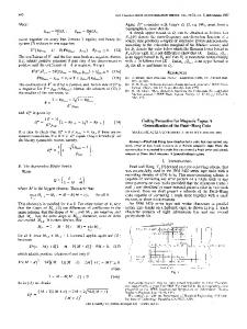
between the two calibration methods used by Holzapfel and Franck/8 •19 suggests that the earlier melting curve is close to correct up to ,_,70 kbar, but that the pressures above this were overestimated by 10%-20%. A correction such as this is necessarily quite uncertain/9 but it seems to us to be at least in the right direction. The corrected, but approximate, melting curve is shown in Fig. 4. The points can be fitted by the Simon equation in the form

P- 22= 6.429[( T/354.8) 4 ·54L 1], with a standard deviation of 5.7°C. There has been some controversy about the reality and explanation of an inflexion in the shock Hugoniot of water at 115 kbar, found by Al'tshuler et al. 20 but

THE JOURNAL OF CHEMICAL PHYSICS

CLARK

not by Walsh and Rice21 or Zel'dovich. 22 A comparison23 of the melting curve of ice VIP with the pressuretemperature curve for shock waves moving into water showed that the two curves meet only in the narrow range between 30 and 45 kbar. The present correction of the melting curve of ice VII does not affect this conclusion. ACKNOWLEDGMENTS The authors would like to thank Mrs. Martha C. Pistorius for writing the computer program used in fitting the data. J. Erasmus and his staff and G. O'Grady and his staff kept the equipment in good repair, and were responsible for the manufacture of the furnace parts. Calculations were carried out on the IBM System 360 of the National Research Institute for Mathematical Sciences. 21

E. U. Franck (private communication). 2o L. V. Al'tshuler, K. K. Krupnikov, B. N. Lebedev, V. I. Zhuchikhin, and M. I. Brazhnik, Zh. Eksp. Teor. Fiz. 34 1 874 (1958) [Sov. Phys.-JETP 7, 606 (1958)]. 19

AND

J. M. Walsh and M. H. Rice, J. Chern. Phys. 26,815

(1957). Y. B. Zel'dovich, S. B. Kormer, M. V. Sinitsyn, and K. B. Yushko, Dokl. Akad. Nauk SSSR 138, 1333 (1961) [Sov. Phys.Dokl. 6, 494 (1961)]. 23 S.D. Hamann, Advan. High Pressure Res. 1, 85 (1966). 22

VOLUME 48, NUMBER 12

!5 JUNE !968

Numerical Solution of Quantum-Mechanical Pair Equations* VINCENT

McKoY

AND

N.

W. WINTER

Gates and Crellin Laboratories of Chemistry, t California Institute of Technology, Pasadena, California

(Received 26 January 1968) We discuss and illustrate the numerical solution of the differential equation satisfied by the first-order pair functions of Sinanoglu. An expansion of the pair function in spherical harmonics and the use of finite difference methods convert the differential equation into a set of simultaneous equations. Large systems of such equations can be solved economically. The method is simple and straightforward, and we have applied it to the first-order pair function for helium with 11r12 as the perturbation. The results are accurate and encouraging, and since the method is numerical they are indicative of its potential for obtaining atomicpair functions in general.

INTRODUCTION

In the Hartree-Fock approximation each electron moves in a potential averaged over the motions of all others. This is an excellent starting point, and a great deal of chemical knowledge can be obtained this way. Many properties require more accurate wavefunctions for their prediction and understanding. The difference between the Hartree-Fock and exact wavefunction is referred to as the correlation wavefunction. It is important to have methods of finding the correlation wavefunction and its effect on physical observables. Sinanoglu1 has developed a many-electron theory of atoms and molecules. This theory can provide the wave-

* Supported in part by a t Contribution No. 3642.

grant from the NSF (GP 6965).

1 Some early references are 0. Sinanoglu in J. Chern. Phys. 33, 1212 (1960); Phys. Rev. 122, 493 (1961); Proc. Roy. Soc. (London) A260, 379 ( 1961); Proc. Nat!. Acad. Sci. U.S. 47, 1217 (1961). For a review of the theory and an extensive list of references see 0. Sinanoglu, Advan. Chern. Phys. 6, 315 (1964).

function and energy of an atom or molecule to chemical accuracy, and it does so in such a way that it does not become rapidly difficult or uneconomcial as the number of electrons increases. In one of his early papers1 the first-order correction to the single-particle wavefunction was expressed in terms of pair functions which describe the correlation between pairs of electrons. 2 These firstorder pair functions are solutions of nonhomogeneous partial differential equations. The equations are just like those for an actual two-electron system, except that each electron moves in the Hartree-Fock (HF) field of the entire medium. This has not been fully appreciated, especially from a computational standpoint. Each pair energy has a variational principle, and attempts to solve the pair equations have been mainly 2 In later papers the pair theory was made accurate .to all o.rde~s, i.e., beyond first order. We refer the reader to the review article m Ref. 1. The complete form of the many-electron theory is not a perturbation theory.

Downloaded 14 Feb 2006 to 131.215.225.176. Redistribution subject to AIP license or copyright, see http://jcp.aip.org/jcp/copyright.jsp

5515

QUANTUM-MECHANICAL PAIR EQUATIONS

by this method. The variational method reduces the calculation to the evaluation of a large number of integrals. The presence of a nonlocal potential in the HF operator does lead to some difficult integrals, which can become more difficult if higher powers of the interelectronic coordinate are included. A large effort has gone into evaluating such atomic integrals. In this paper we discuss and illustrate the numerical solution of the differential equation satisfied by a pair function. An expansion of the pair function in spherical harmonics and the use of finite· difference methods convert the differential equation into a set of simultaneous equations. Large systems of such equations can be solved quite economically, e.g., about 2000 equations in two minutes. The method has many attractive features, and we have applied it to the equation of the first-order pair function for the helium atom. The results are accurate and encouraging, and since the method is numerical, these results are truly indicative of its potential in solving for atomic pair functions in general.

THEORY The total Hamiltonian, H, and the zeroth-order Hamiltonian, Hn, for anN-electron atom are

L N

i=1

(

~ + LN 1 -!Vf-r;

iN ), (9) where 'l1;}1l (x;, X;), a first-order pair function, satisfies the nonhomogeneous differential equation

A. Sinanoglu's Pair Equations

H=

equation

( 1)

(e,+ei)-a;pl = -Q(1/r12) B(~j>,(l)!f>i(2) ).

( 10)

The operator, Q, makes a two-electron function orthogonal to all occupied H-F orbitals; i.e., N

Q= 1-

and

2: •C1> )(4>;(1) 1+14>•(2) )(4>,(2) I> i-1

N

Ho=

L

(h, 0+V,),

N

(2a)

+

i=1

respectively. In Eq. (2a) V; is the Hartree-Fock potential, which is the same for all electrons. For closed-shell is uniquely defined. 3 Also in Eq. (2a), atoms

v,

L

IB(4>;(1)4>i(2) ))(B(!j>;(1)4>,(2) )I,

(11)

i(x1, x2) ).

(15)

i, is the solution of the first-order part of the Schri:idinger equation for two electrons in the HF "sea." The effect of the medium enters through the HF potentials in the operators e; and Q. One can write the solution of Eq. (10) as follows:

(22) (23)

andif;(l> satisfiesEq. (6). ComparisonofEqs. (6), (21), (22), and (23) shows that if;(l) is just an example of a pair function. This is the example we use to illustrate our method of solution of pair equations. Numerical details of the method demonstrate that these results are indicative of its usefulness for obtaining atomic pair functions in general. B. Reduction of Pair Equations For quantitative results one must solve Eqs. (10), (17), or (21). Most attempts so far have used a varia-

tional approach. Equation (15) can be written

(16) where Q is defined in Eq. ( 11) and u 0 satisfies the equation

(e,+e1)u;;= [1;1- K,i- (1/r12) ]B(~/~;(1)1/1;(2) ),

(18) •=1

where 1/1;/ are unperturbed pure symmetry states. Then, m

.2: a.u;]

( 19)

-1

(e,+e1)u;;"= [ (1/1;/( 1/r12 )1jl;;')- (ljr 12 ) ]1/1;/.

(20)

The solution of Eq. (10) does not require any vector coupling schemes such as Eqs. (18) and (20), but the obvious symmetry properties of U;/ are convenient if u;1 is expanded in spherical harmonics. We have given Eqs. (17) and (20) because the use of symmetry pairs leads to simplifications in the numerical treatment of these equations. Equation ( 17) is also very similar to the equation one obtains starting from a bare nuclei Hamiltonian, i.e., a hydrogenic y;. In that case, the first-order wavefunction is again written like Eq. (9) but with a;p> replaced by U;;, which satisfies an equation very similar to Eq. (17), i.e.,

[ -!v?- V22 -

(Z/r 1 ) - (Z/r2 ) -e;-e;]u;;

= [J,;- K;1- (ljr12 ) ]B(q,;( 1)q,j(2) ).

(21)

=

.2:

(24)

E;/2) l

i, i.e.,

( 17)

with f;; and K,1 the Coulomb and exchange integrals for orbitals ljl; and 1/1;. This approach has some advantages if one needs to expand U; 1 in a series of spherical harmonics. The general solution to Eq. ( 17) is obtained by orthogonalizing a particular solution to B(q,, r/>;). If B(~/~;(1)1/1;(2)) belongs to a two-electron irreducible representation, then Eq. (17) has a unique solution, e.g., 1s2 pair of electrons. However, when B(q,;(l)q,1(2)) is not a pure two-electron symmetry state, then Eq. (16) does not have a solution,! and one must write

u;;=

£(2)

e;}2l~e;/< 2 >

= 2(B(r/>;r/>;), m;111;/)

+ ('11;/(1>, ( e;+e;)'l1;/< i), 1

(25)

with

m;1(1, 2) =(1/r12 )-Si(1)-S;(2)-S;(2) - S;( 1) +l;;- K;;,

S;(1) =S;(l)-R;(1),

(26a) (26b)

and '11;/ is varied to minimize e;/. With a variational form for 'l1;/l+t s,.,.

and is a surface harmonic. Substitution of the expansion Eq. (27) into Eq. (17) or Eq. (10) gives

X (rtr2)- 1fl~m:l'm'Crt, r2) S,m(6~, c~Jt) Sz•m•C62, c~J2).

(29)

For closed-shell systems the Hartree-Fock potential, V(r1 ), is spherically symmetric. For open-shell systems one still requires the potential to be spherically symmetric and the orbitals, symmetry orbitals.8 With the expansion, Eq. (28), the right-hand side of Eq. (10) or Eq. (17) becomes a sum of terms,

2:

Gzml'm'(rt, r2)S1m(1) s,,m,(2).

ll'mmf

The Gzm:l'm' are combinations of terms U 1(r1, r2) and the radial factors of the H-F orbitals. One now obtains a set of uncoupled equations, one for each term in Eq. ( 27), (30)

In deriving Eq. ( 30) we have used relationships such as S;;(O, q,) Skz(O, q,) =

2: ai;klallSafl(O, q,),

(31)

In operator notation Taylor's series can be written5

y(x+h) =y(x) +h(dy/dx) +th2 (rJ2y/dx2)

a(l

where a;;~c 1all are numerical coefficients. Equation (30) is our basic equation. It is a second-order elliptic partial differential equation in two variables, and no closedform solution exists.

= exp(hD)y(x).

(32a)

Define a central difference operator o,

oy(x+th) =y(x+h) -y(x)'

(32b)

and one has the operator equation

C. Analysis

Of the numerical methods for solving partial differential equations, those employing finite differences are most frequently used. Finite-difference methods are approximate in the sense that derivates at a point are approximated by difference quotients over a small interval; i.e., aq,jax is replaced by &pjox where ox is small, but the solutions are not approximate in the sense of being crude estimates. In these methods the area of integration is divided into a set of square meshes, and an approximate solution to the differential equation is found at these mesh points. This solution is obtained by approximating the partial differential equation by n algebraic equations. The values at the mesh points form a vector which is the solution of the set of simultaneous linear equations. A numerical solution contains no arbitrary constants, so that we always obtain particular integrals rather than complete primitives of the differential equation.

+ ••·

o= exp(thD)- exp( -thD) =2sinh(thD), and hence

(32c)

h2V= (2 sinh-1to) 2

=o2--fio4+-JtrOL....

(33)

The second derivative of a function at the ith point is

The operators o2 and o4 , etc., are defined by the equations

1i2y(x) =y(x+h) +y(x-h) -2y(x),

(35)

/i 4y(x) =y(x+2h) -4y(x+h)+6y(x)

-4y(x-h)+y(x-2h).

(36)

'See, for example, L. Fox, The Numerical Solution of Two-Point Boundary Problems in Ordinary Differential Equations (Oxford University Press, New York, 1957).

Downloaded 14 Feb 2006 to 131.215.225.176. Redistribution subject to AIP license or copyright, see http://jcp.aip.org/jcp/copyright.jsp

5518

V. McKOY AND N.

Here, his the spacing between neighboring mesh points, and the partial derivatives of Eq. (30) become h2[(a 2jax2)

+ (a jay) ]u(x, y) 2

= (o.,2+o,,2)u(x, y) - /2 (o.,4+o,i)u(x, y) +O(o6).

(37)

At a point u(x, y) one has

[(a 2jax 2) + (a 2jay) ]u(x, y)

= (1/h2) [u(x+h, y)+u(x-h, y)+u(x, y+h) +u(x, y-h) -4u(x, y) ]+Cu(x, y),

(38)

with C=- (1/12h2) (ox4+oy4)

+ (1/90h

2

)

(o.,6+oy6 ) - • • ••

(39) As a first approximation we neglect Cu in Eq. (38) and therefore replace the differential operator by the first term on the right-hand side. This leads to a truncation error in the expansion of the differential operator. The form of this truncation error is important, as it allows us to predict the convergence of the numerical solution as one approaches the exact solution (see Appendix A). From Eqs. ( 33 )-( 39) it is obvious that the local truncation error in the second-difference approximation is O(h2 ). The term Cu in Eq. (39) contains higher difference operators, which can be included by an iterative technique (see Appendix B) . One must now specify the boundary conditions for Eq. (30). We treat the problem as a boundary-value one, specifying the value of the solution on a boundary enclosing the area of integration (Dirich!et boundary conditions). The functions Uzm:!'m'(l) vamsh along the boundaries r 1= 0, r2 = 0. These functions also vanish as r1 or r2~ oo. This boundary condition must be modified so as to handle the equation on a finite numerical grid. There are two alternatives, and both are based on the condition that the solutions approach zero exponentially and essentially do so at some finite value of the independent variable. One can choose a value of r1 = R1 and make the solution vanish on this boundary, i.e., u(R1, r2 ) =u(r1, R 1) =0. One then moves this boundary out to r 1 =R2, R 3, etc., until at least two adjacent values at the boundary are zero to the required number of significant figures. The boundary condition is then accurately satisfied. The other alternative is based on the asymptotic form of the solution of Eq. ( 30) . We can use this as a boundary condition. For large values of r1 and r2 the solution behaves like g(r1, r 2 ) exp[ -a(r1+r2) ], where g(r 1, r 2 ) varies slowly. This behavior becomes a boundary condition, ( 40)

The boundary condition is satisfied when Eq. (40) holds between neighboring points. Both alternatives work

W. WINTER

well and bring all atoms of interest within reach of the method. With Eq. (38) the differential equation is obviously replaced by a set of algebraic equations. In matrix form these equations are ( 41) Au=b, where u is a column vector, the components of which are approximate solutions to the differential equation at a set of internal points. Were it not for the nonlocal exchange potentials of Eq. (30) [see Eqs. (13b) and (14b)], the matrix A, Eq. (41), would have a very simple structure; e.g., forM divisions along each dimension the only nonzero elements lie on the diagonal, the super-, and sub-diagonal, and on lines parallel to the diagonal but M strips above and below the diagonal. This is a banded matrix of half-bandwidth equal toM. We now show that (a) large systems of such equations can be solved rapidly and accurately, and (b) once such solutions have been obtained, the nonlocal operators can be taken into account with a small increase in computing time. We put more emphasis on (a), but (b) is shown quite convincingly. For B internal points in each dimension we have N equations with N =B 2. The matrix A then has dimensions B2XB2 ; e.g., with B about 40 one has a 1600X 1600 matrix. We use the method of triangular resolution to solve the matrix equation, Eq. (41). The method has been efficiently programmed,6 and very large systems of equations can be solved economically. We give a very brief outline of the method. If the leading minors of the matrix A are nonzero, there is a unique lower triangular matrix Land a unique upper triangular matrix U so that A=LU. An upper triangular matrix is one which has zeros above the diagonal. The solution proceeds by eliminating the lower triangular elements, taking pivots successively along the principal diagonal, and the only recorded quantities are the multipliers needed for the triangular resolution (L) and the triangularized array (U) . The band structure is preserved in the L and U factors. 7 Solution of the linear equations is straightforward; i.e., for Ax:=b one solves Ly=b and Ux=y by forward and backward substitution. The L and U matrices can be used to operate on any number of righthand vectors, 8 i.e., b of Eq. ( 42). 6 It can be shown that there is no limit on the number of rows of equations that can be handled and that the ~ppe~ limit on t~e bandwidth is set by the requirement of havmg ·2 t.erms m memory at any one time. For an IBM 7094 an upper hm1t t~ the M is about 200. This corresponds to a large number of equatiOns. For details of the program see C. W. McCormick and K. J. He bet, "Solution of Linear Equations with Digital Computers," Tech. Rept., Engineering Division, California Institute of Technology, 1965 (unpublished) . . . . . 7 L. Fox, Numerical Solution of Ordznary and Partzal Differentzal Equations (Pergamon Press, Inc., London, 1962) .. ' Most of the computing time is required to o~tam ~he Land U factors and the time to forward- and back-substitute IS much less. This feature enables us to include, by an iterative scheme, both nonlocal potentials and higher-order differences. See Appendix B for details.

M:

Downloaded 14 Feb 2006 to 131.215.225.176. Redistribution subject to AIP license or copyright, see http://jcp.aip.org/jcp/copyright.jsp

QUANTUM-MECHANICAL PAIR EQUATIONS

For a method to be practical the computing-time requirements must be realistic. The real advantage of triangular resolution for band matrices is that the running time for inversion of an NXN matrix is proportional to N 3 rather than JPN for triangular resolution. M is the half-bandwidth. For this differential equation N-;:::::,M2 , and the ratio of running times for matrix inversion to triangular resolution is M 2• Matrix inversion does not preserve band structure, and the time to determine a new set of roots, i.e., solve Eq. ( 40) with a new vector b, is proportional to N 2• The time savings involved here are significant, e.g., a factor of 1600 for M-;::::::,40. In the next section we give an example which shows that the method is numerically and economically feasible. RESULTS When the differential equation is converted into a set of simultaneous linear equations the term Vch) [see Eq. (14a)l is just an algebraic operator evaluated at every mesh point on the grid. For H-F orbitals one would evaluate integrals such as Si(r 2 ), Eq. (13a), analytically and tabulate them at the necessary points.

5519

For a numerical method it makes no difference to the analysis whether the potential term, Vc(ri), in Eq. (30) is given by HF orbitals or is just the electron-nucleus attraction, i.e., hydrogenic zeroth-order Hamiltonian. They both give rise to numerical arrays, which are evaluated even before the numerical analysis really begins. Hence, to demonstrate our method we pick the simplest pair equation, that for the helium atom starting from a hydrogenic H 0 • The important issue here is the practicality of solving the number of simultaneous equations which must be solved so as to obtain an accurate value of a pair energy. Also, for helium we have a series of previous results on the energy contribution of each partial wave to the second-order energy. Consider Eqs. (21) and (27). For a Ui; of S symmetry only those Uzm:l'm' with l=l' are nonzero, and U!m:l'-m is independent of m. This gives the partial wave expansion, u( 1s2 )

=

~ LJ 1=0

uz(rl, r2) Pz( cos812). r1r2

(42)

Recall that u(1s 2 ) must be made so that (u(1s 2 ), B(lsa1stl) )=0. The differential equations are

(43)

(44)

for l=O and 1?_1, respectively, and (45)

P1.(r) =rR1s(r).

In Eqs. ( 43) and ( 44) we have €18 =- 2.0, Et = 1.25, and Rlt=4V2e2'. Tables I and II give the results for the first three partial waves. Here the second-order energy

l ! i1

7

l

~

to

E2(l=O) = (Uo(rl, r 2), (1/ri2)B(1s(1) 1s(2) )) -EI(Uo,B(1s(1)1s(2))),

(46a)

E2(l?: 1) = (uz(r1, r2), ( 1;r12) B(1s(1) 1s(2) )). ( 46b)

TABLE I. Results for the l =0 partial wave of the helium pair function. •

Mesh sizeb

decouples into a sum over the partial wave contributions, E2(l). All integrations are done by the trapezoidal rule, and

Number of equations•

E2(l=O)

Execution time (seconds on IBM 7094)

361 576 841 1156 1521 1936 2401

-0.12605 -0.12678 -0.12664 -0.12640 -0.12619 -0.12603 -0.12591

3d 16• 27 52 82 115 169

• See Eq. (43). The perturbation is l/r12. b Spacing between grid points. c Number of points at which an approximate solution to the differential equation is obtained. d This size problem fits completely in random access memory. e This size problem requires auxiliary disk storage.

In Tables I and II we have given the computing times necessary to solve the equations at each mesh size. We feel it is important to communicate the computing needs of a given method. Computing times for this method are quite low. For l=O we require u(r~, r 2) to vanish at R=5 and obtained the solutions at seven different mesh sizes: h=!,t,i,i-, t,t,lo- To test the boundary condition we allowed u(r1, r2) to vanish at R=6 and, at a mesh size of t, found E 2 (l=O) =-0.12607, compared to -0.12605 for the same condition at R=S. With the exponential behavior of the function as a boundary condition at R=S we obtained E 2 (l=O) =-0.12607, while at R=4 one finds E 2 (l=O) =-0.1261. The boundary condition poses no difficulty. For h=i there are 361 equations, and the entire problem can be loaded into the random access memory of an IBM 7094 and

Downloaded 14 Feb 2006 to 131.215.225.176. Redistribution subject to AIP license or copyright, see http://jcp.aip.org/jcp/copyright.jsp

5520

V.

McKOY AND N.

TABLE II. Results for the I= 1 and 2 partial waves of the helium pair function. Mesh size

W.

WINTER

TABLE IV. Extrapolants from intermediate meshes.•

&(l=1)

Ez(l=2)

Execution timeb

-0.033051• -0.030387 -0.029073 -0.028333 -0.027874 -0.027569 -0.027356

-0.0056616 -0.0049862 -0.0046351 -0.0044302 -0.0043007 -0.0042137 -0.0041525

3• 12d 23 37 50 82

Mesh size

2•

6

1

1=0

1=1

All integrals evaluated by the trapezoidal rule. b Execution time in seconds on an IBM 7094. 0 This size problem fits entirely in core. d This size problem requires auxiliary storage.

solved within 3 sec. At h = t one requires disk storage to handle the 576 equations, and the execution time is 16 sec. Table II gives the results for l = 1 and l = 2 partial waves. The execution times are lower than those for the l=O case, since the exponential boundary condition could be imposed at R=4 for these higher partial waves. One can expect this behavior for the higher l components of pair functions. Requiring the function to vanish at R = 6 affected the seventh significant figure in the energy. Tables III-V give the results of extrapolating the values at varying mesh sizes (Tables I and II) .In Appendix A we derive the convergence of the solution of the corresponding finite difference equations, u(h), towards the solution of the differential equation itself, u. We show that

(47) TABLE III. Extrapolants from finest meshes.• Mesh size

Results from direct quadrature

h2 extrap-

h4 extrap-

olants•

olantsd

-0.126194b -0.12541 -0.126030

1=0

-0.12531

1=2

~

-0.029073

8

1

-0.027874

n

-0.027356

olantsd

-0.12526 -0.12539

-0.125905

-0.026332 -0.026495 -0.026436

6

1

-0.0046351

i

-0.0043007

1

h4 extrap-

olants• -0.12562

-0.126194

TO

h2 extrap-

-0.126642b

t io 6

8

Results from direct quadrature

-0.0038707 -0.0038996 -0.0038892 -0.0041525

• See Eq. (48) of text. b Results from direct quadrature on numerical solutions (Tables I and II). " Extrapolants from pairs of successive values in the preceding column assuming an h2 convergence. d Extrapolants from the three values in the first column assuming an h" and h4 convergence.

where u, u(h), a2, anda4 are functions of the independent variables and h is the mesh size. We therefore know exactly how an approximate solution approaches the exact one. This convergence property forms the basis of an extrapolation technique which allows us to obtain a high degree of accuracy for the pair energies. We checked the use of Eq. ( 47) by comparing an actual solution with an extrapolated one. The agreement is excellent. The integrals for E2 are evaluated by the trapezoidal rule. The error term for quadrature by the trapezoidal rule can be expressed as a power series in the interval size, h. In Appendix A we show that the second-order energy, evaluated by the trapezoidal rule and with the finite difference solution, converges to the exact value

-0.12537 -0.125905

TABLE V. Extrapolants from values at various meshes.

-0.027874

Values used in extrapolation

-0.026422 -0.027569

I= 1

-0.026498 -0.026449

1

TO

-0.027356

-0.12574 -0.12512 -0.12521

1=0

-0.0043007 -0.0038862 1=2

-0.0042137

-0.003902 -0.0038919

-0.0041525 • See Eq. (48) of text. b Results from direct quadrature on numerical solutions (Tables I and II). c Extrapolants from pairs of successive values in the preceding column assuming an hi convergence. d Extrapolants from the three values in the first column assuming an h' and h• convergence.

=1

(l, !) (!, l) (l, !, !) (!, ••

-0.02564 -0.02609 -0.02645 -0.02649

+l

(l, !) (t, t)

1=2

Extrapolants

(l, !, t) (l, !, t, +l ct ! .... ~.

rol

-0.003786 -0.003837 -0.003878 -0.003896 -0.003905

• The values at these mesh sizes were used in the extrapolation.

Downloaded 14 Feb 2006 to 131.215.225.176. Redistribution subject to AIP license or copyright, see http://jcp.aip.org/jcp/copyright.jsp

5521

QUANTUM-MECHANICAL PAIR EQUATIONS

TABLE VII. Upper bounds derived from numerical salution.•

as follows: E2=E2(h) +b2h2+b4h'+ • · ·,

(48)

where E2 (h) is the energy obtained at each mesh size. With Eq. ( 48) we can derive very accurate extrapolants. To obtain the best results one obviously extrapolates the results from the finer meshes. If one simply wants a good estimate of a pair energy, extrapolation from coarser meshes may be sufficient. Tables III and IV give the extrapolants based on results from the finest meshes, i.e., h=i, t, -ftr and those derived from the results at h=t, t,-ftr, respectively. The various columns of Tables III and IV correspond to an extrapolation from a successively higher-order polynomial, i.e., an h2 and h4 extrapolation. The successive columns of both Tables indicate that the extrapolation is stable and yields excellent results. Table V lists extrapolants derived from the results at various mesh sizes. We do this primarily to show the kind of extrapolant!:> one can obtain from results at cruder meshes. These compare well with the best results of Table III. This approach can yield useful estimates of pair correlation energies. For the l = 1 partial wave extrapolation from mesh sizes t, k, ~ give -0.02645. These solutions were obtained with a total computing time of 17 sec. Table V also lists some extrapolants based on very high-order polynomials; e.g., use of the results at all seven mesh sizes implies an h10 extrapolation and for l = 2 gives E2(l=2) =-0.003905. Other extrapolants indicate a similar stability. For comparison we use the most recent results on the helium-atom pair function. Byron and Joachain9 solved the pair equation variationally and also gave the contributions of the various partial waves to E2. They used two different types of trial functions. For u 1( r1, r2) of Eq. ( 42) they chose (a) a "configuration-interaction" type expansion, 1tl(rt,

r2) =

L Clmn(Ytmr2"+rtny2m) m,n

Xr1r2 exp[- 2(r1+r2) ],

( 49a)

and (b) a function of the form uz( Yt, r2) LClmnYtY2r>my;( 1)¢;(2) )-Qm;;u;;.

I= T(h) +ah4+0(h6 ),

~;,=B(cJ>.,(1)ct>1 (2) )+u;;.

(56)

(57) Neglecting the second term on the right-hand side, Eq. (57) becomes identical with Eq. (10) for u;/1). An obvious approach to the solution of Eq. (57) would be iterative; i.e., take u;/1) and use the L and U matrices to solve for AU;; due to the term Qm;;u;; [see discussion below Eq. (52)]. The algebra on the spherical harmonics may be more involved, but comparison between u;p> and u;i> Eq. (57), will be informative.

APPENDIX A An advantage of the numerical method is that one can derive the convergence of the numerical solution, u(x, y, h), towards the exact solution, u(x, y). One expands u(x, y),

u(x, y) =u(x, y, h)+Ah+Bh2+Ch3+ .. ·,

(A1)

where A, B, C, • • ·, are functions of x and y. The differential equation, Eq. (30), has the form

f(D)u=g(x, y),

(A2)

f(D) = -t(c'J2fax2) -!(82/8y2) +p(x, y),

(A3)

where

where T(h) is the value of the integral evaluated by the trapezoidal rule. Use of the numerical solution, instead of the exact solution, to evaluate T(h) introduces terms proportional to h2, h4, etc., into Eq. (A12). The final form is

APPENDIX B In Eq. (38) we neglected the term Cu and retained just the second difference operator. Instead of going to very fine meshes one may include fourth differences, e.g., Eq. (36), and this may give an accurate solution at coarser meshes.7 Consider the first term of Eq. (39), C=-(1/12h2)(o,4+o114),

(A4)

Lu(h) =[j(D)+(ch2+dh4+· • · )]u(h). (AS) Substituting for u(h) and equating powers of h,

f(D)u=g(x,y),

(A6)

j(D)A=O,

(A7)

f(D)B-cu=O,

(A8)

f(D)C+cA =0.

(A9)

Note that Eq. (AS) has its form due to the use of central differences. From Eqs. (A7) and (A9) A and Care zero. Thus, Eq. (Al) becomes (A10) 0. Sinanoglu (private communication).

(B2)

(A+C)y=b.

The matrix A dominates, and for a first approximation, y{l), one has Ay requires values of the function beyond the boundaries [see Eq. ( 36)]. One often extrapolates across the boundary, but there is an apparent indeterminacy at the boundary [see Eq. ( 43)]. One can derive a relation between the point next to the boundary and the first external one through a cusplike condition. In the region r1>r2let x=r1, y=r2, and ~0; we have 2 2 1 1 1) £\ - 2 ax2 Xi - 2 ay2 y-+{) y-.Q =O,

(a u)

(a u)

[(l(l+

+ 2T -

;rJ

(B5) Substitution from Eq. (35) into Eq. (BS), and with

(aujay)u,= {[u(x, Y2+h)-u(x, y2-h)]/2hl+O(h2), (B6) one obtains the necessary relationship. The limits (ujy) 71 -+{J and (u/y2l 71-o are evaluated using L'Hopital's rule for indeterminate forms.

Downloaded 14 Feb 2006 to 131.215.225.176. Redistribution subject to AIP license or copyright, see http://jcp.aip.org/jcp/copyright.jsp