Observer Design for Time Delay Nonlinear Triangular ...

Observer Design for Time Delay Nonlinear Triangular Systems Boubekeur Targui, Carlos Manuel Astorga-Zaragoza, Miloud Frikel, Mohammed M’Saad, Eric Magarotto

To cite this version: Boubekeur Targui, Carlos Manuel Astorga-Zaragoza, Miloud Frikel, Mohammed M’Saad, Eric Magarotto. Observer Design for Time Delay Nonlinear Triangular Systems. 18th IFAC World Congress, Aug 2011, Milan, Italy. 6 p.

HAL Id: hal-01063155 https://hal.archives-ouvertes.fr/hal-01063155 Submitted on 11 Sep 2014

HAL is a multi-disciplinary open access archive for the deposit and dissemination of scientific research documents, whether they are published or not. The documents may come from teaching and research institutions in France or abroad, or from public or private research centers.

L’archive ouverte pluridisciplinaire HAL, est destin´ee au d´epˆot et `a la diffusion de documents scientifiques de niveau recherche, publi´es ou non, ´emanant des ´etablissements d’enseignement et de recherche fran¸cais ou ´etrangers, des laboratoires publics ou priv´es.

Observer design for time delay nonlinear triangular systems B. Targui*, CM. Astorga-Zaragoza**, M. Frikel*, M. M’Saad*, E. Magarotto* ∗

Groupe de Recherche en Informatique, Image, Automatique et Instrumentation de Caen, UMR 6072, 6 Boulevard du Marechal Juin, 14050, Caen Cedex, France. (Email: [email protected], Tel. +33(0)2 31 45 27 12, Fax: +33 (0)2 31 45 26 98) ∗∗ Centro Nacional de Investigacin y Desarrollo Tecnol´ ogico, Interior Internado Palmira s/n, Col. Palmira, C.P. 62490, Cuernavaca, Mor., Mexico Abstract: In this work an observer for a class of delayed nonlinear triangular systems with multiple and simple time-delay is proposed. The main feature of this observer is that it is easy to implement because of its constant gain. First, the observer synthesis is presented for nonlinear systems with variable time-delay and is extended for nonlinear systems with multiple time-delay. The observer performance is evaluated through numerical simulations.

Keywords: nonlinear time-delay systems, nonlinear observers, triangular forms. 1. INTRODUCTION In the recent years time-delayed systems have been investigated extensively because of the delay phenomenon is often encountered in various engineering systems such as mechanical and electrical systems, communication networks, among others. The source of a time-delay may be due to the nature of the system or induced into the system due to the transmission delays associated to other components interacting with the system. A time-delay may be the origin of instability or oscillations in a system. For this reason, many researchers are devoted to investigate the different fields of automatic control for time-delayed systems, such as stability, observability, controllability and system identification, among others. For instance, in Richard (2003), different control approaches for delayed systems are presented. The case of observer design for state estimation of nonlinear systems is treated by many authors from a theoretical and practical point of view, see for instance, Gauthier et al. (1992), Gauthier and Kupka (1994), Targui et al.(2002), Farza et al. (2004). The observer synthesis for triangular nonlinear systems is related to the notion of uniform observability, for instance, the authors in Targui et al.(2002), propose a high-gain observer with constant gain for nonlinear systems having a triangular structure and a single output. In Targui et al. (2001), a generalization for multipleoutput systems is presented. A lot of researchers, such as Darouach (2001), Hou (2002), Wang et al. (2002), have extensively investigated the case of observer synthesis for delayed systems. For instance, in Germani et al. (2002), a chain of observation algorithms reconstructing the system state based on delayed measurements of the process output is proposed. In Ibrir (2009), an adaptive observer for time-

delay nonlinear systems in triangular form is presented. This paper is organized as follows. Section 2 is devoted to preliminaries and the problem formulation. Section 3 describes the observer synthesis for a class of nonlinear systems with a signal variable time-delay. An extension of this observer for nonlinear systems with multiple and variable delays is presented in Section 4. In Section 5 numerical simulations are presented in order to evaluate the observer performance and finally conclusions are discussed in Section 6.

2. PRELIMINARIES AND PROBLEM FORMULATION Consider the following non-linear delayed system: ⎧ 𝑥˙ 1 = 𝑓1 (𝑢, 𝑢𝜏 , 𝑥1 , 𝑥1𝜏 , 𝑥2 )     𝑥˙ 2 = 𝑓2 (𝑢, 𝑢𝜏 , 𝑥1 , 𝑥1𝜏 , 𝑥2 , 𝑥2𝜏 , 𝑥3 )    ..    .  ⎨ 𝑥˙ 𝑖 = 𝑓𝑖 (𝑢, 𝑢𝜏 , 𝑥1 , 𝑥1𝜏 , 𝑥2 , 𝑥2𝜏 , . . . , 𝑥𝑖 , 𝑥𝑖𝜏 , 𝑥𝑖+1 ) .    ..     𝑥˙ 𝑛−1 = 𝑓𝑛−1 (𝑢, 𝑢𝜏 , 𝑥1 , 𝑥1𝜏 , . . . , 𝑥𝑛−1 , 𝑥𝑛−1𝜏 , 𝑥𝑛 )     ⎩ 𝑥˙ 𝑛 = 𝑓𝑛 (𝑢, 𝑢𝜏 , 𝑥, 𝑥𝜏 ) 𝑦 = 𝑥1

(1)

where 𝑢(𝑡) ∈ ℝ𝑚 and 𝑦 ∈ ℝ are the input and the output ⎡ ⎤ 𝑥1 (𝑡) ⎢ 𝑥2 (𝑡) ⎥ 𝑛 ⎥ of the system. 𝑥(𝑡) = ⎢ ⎣ ... ⎦ ∈ ℝ is the state vector. 𝑥𝑛 (𝑡) Henceforth the next notations are used

⎤ ⎡ 𝑥1𝜏 𝑥1 (𝑡 − 𝜏 (𝑡)) ⎢ 𝑥2 (𝑡 − 𝜏 (𝑡)) ⎥ ⎢ 𝑥2𝜏 ⎥=⎢ . 𝑥𝜏 (𝑡) = 𝑥(𝑡 − 𝜏 (𝑡)) = ⎢ .. ⎦ ⎣ .. ⎣ . ⎡

where 𝑠𝑖𝑖 > 0 and 𝑠𝑗 < 0; 𝑖 = 1, . . . , 𝑛; 𝑗 = 1, . . . , 𝑛 − 1.

⎤ ⎥ ⎥ ∈ ℝ𝑛 , ⎦

𝑥𝑛𝜏 𝑥𝑛 (𝑡 − 𝜏 (𝑡)) 𝑢𝜏 (𝑡) = 𝑢(𝑡 − 𝜏 (𝑡)), where 𝜏 (𝑡) a known variable delay and 𝑥(𝑡) = 𝜙(𝑡) for 𝑡 ≤ 𝜏 . 𝜙(𝑡) is the initial condition belonging to a Banach space and ∥ ⋅ ∥ represents the Euclidian norm of a vector. System (1) can be written in the following form: { 𝑥(𝑡) ˙ = 𝑓 (𝑢(𝑡), 𝑢𝜏 (𝑡), 𝑥(𝑡), 𝑥𝜏 (𝑡)) (2) 𝑦(𝑡) = 𝐶𝑥(𝑡) where ⎤ ⎡ 𝑓1 (𝑢, 𝑢𝜏 , 𝑥1 , 𝑥1𝜏 , 𝑥2 ) 𝑓2 (𝑢, 𝑢𝜏 , 𝑥1 , 𝑥1𝜏 , 𝑥2 , 𝑥2𝜏 , 𝑥3 ) ⎥ ⎢ ⎥ ⎢ .. ⎥ 𝑓 =⎢ . ⎥ ⎢ ⎣𝑓 (𝑢, 𝑢 , 𝑥 , 𝑥 , . . . , 𝑥 ,𝑥 ,𝑥 )⎦ 𝑛−1

𝜏

1

1𝜏

𝑛−1

𝑛−1𝜏

∙ Define the (𝑛 × 𝑛) diagonal matrix Λ𝜌 as [ ] Λ𝜌 = 𝑑𝑖𝑎𝑔 𝜌, 𝜌2 , . . . , 𝜌𝑛 where 𝜌 is a strictly positive real number.

Lemma. (Targui et al.(2002)). There exist an 𝑛 × 𝑛 constant symmetric positive definite matrix 𝑆 having the form given in Equation (6) and a strictly positive real number 𝜂 > 0, such that 𝐴𝑇 (𝑡)𝑆 + 𝑆𝐴 − 2𝐶 𝑇 𝐶 ≤ −𝜂𝐼; ∀𝑡 ≥ 0 (8) where 𝐴 is given by Equation (5) and 𝐼 is the (𝑛 × 𝑛) identity matrix. The elements of 𝑆, i.e. 𝑠𝑖𝑖 , 𝑠𝑗 , 𝑖 = 1, . . . , 𝑛; 𝑗 = 1, . . . , 𝑛 − 1, are given in function of 𝛼 and 𝛽 defined in Equation (4).

𝑛

𝑓𝑛 (𝑢, 𝑢𝜏 , 𝑥, 𝑥𝜏 ) and 𝐶 is a (1 × 𝑛) matrix: 𝐶 = [ 1, 0, . . . , 0 ] (3) The following assumptions are introduced: Assumption 1 (A1). The functions 𝑓𝑖 ; 𝑖 = 1, . . . , 𝑛 are globally Lipschitz w.r.t. 𝑥 and 𝑥𝜏 , then ∃ 𝑐 > 0 and ∀ 𝑥(𝑡), 𝑦(𝑡), 𝑥(𝑡 − 𝜏 ), 𝑦(𝑡 − 𝜏 ) ∈ ℝ𝑛 such that: ∣∣𝑓 (𝑢, 𝑢𝜏 , 𝑥, 𝑥𝜏 ) − 𝑓 (𝑢, 𝑢𝜏 , 𝑦, 𝑦𝜏 )∣∣ ≤ 𝑐(∣∣𝑥 − 𝑦∣∣ + ∣∣𝑥𝜏 − 𝑦𝜏 ∣∣) Assumption 2 (A2). Assume that the functions 𝑓𝑖 (.), 𝑖 = 1, . . . , 𝑛 − 1 satisfy.

(7)

3. OBSERVER SYNTHESIS Consider the following dynamical system: 𝑥 ˆ˙ = 𝑓 (𝑢(𝑡), 𝑢𝜏 (𝑡), 𝑥 ˆ(𝑡), 𝑥 ˆ𝜏 (𝑡)) − Λ𝜌 𝑆 −1 𝐶 𝑇 (𝐶 𝑥 ˆ(𝑡) − 𝑦(𝑡)) (9) where 𝑆 is given by Equation (6) and satisfies the precedent Lemma; 𝐶 is given by Equation (3); ⎡ ⎤ 𝑥 ˆ1 ˆ2 ⎥ ⎢𝑥 ⎥ 𝑥 ˆ(𝑡) = ⎢ ⎣ ... ⎦ 𝑥 ˆ𝑛

∂𝑓𝑖 0 < 𝛼 < 𝑎𝑖 = (𝑢, 𝜉) ≤ 𝛽; ∂𝑥𝑖+1 𝑖 = 1, . . . , 𝑛 − 1, ∀𝜉 ∈ 𝑅𝑛

and

(4) Assumption 3 (A3). The variable delay 𝜏 (𝑡) is bounded, e.g. 0 < 𝜏 (𝑡) ≤ 𝜏𝑚𝑎𝑥 , it is differentiable and satisfies 𝜏˙ (𝑡) ≤ 𝜇 < 1. The following notations are employed: ∙ 𝐴 is a (𝑛 × 𝑛) matrix having the following form: ⎛ ⎞ 0 𝑎1 0 . . . 0 .. ⎟ ⎜ ⎜ 0 0 𝑎2 . ⎟ ⎜. ⎟ 𝐴=⎜. (5) .. ⎟ . 0 ⎟ ⎜. ⎝ ⎠ 0 . . . 0 𝑎𝑛−1 0 ... 0 0 where the functions 𝑎𝑖 ; 𝑖 = 1, . . . , 𝑛 − 1 are defined in Equation (4) and each one satisfies Assumption (A2). ∙ 𝑆 is a (𝑛 × 𝑛) constant matrix having the form: ⎛ 𝑠11 𝑠1 ⎜ ⎜ 𝑠1 𝑠22 ⎜ ⎜ 𝑆 = ⎜ 0 ... ⎜ ⎜ . ⎝ .. 0 ...

symmetric positive-definite 0 .. .

0

⎞

⎟ 0 ⎟ ⎟ .. ⎟ . ⎟ ⎟ ⎟ .. . 𝑠𝑛−1 ⎠ 0 𝑠𝑛−1 𝑠𝑛𝑛

⎤ 𝑥 ˆ1𝜏 ˆ2𝜏 ⎥ ⎢𝑥 ⎥ 𝑥 ˆ𝜏 = 𝑥 ˆ(𝑡 − 𝜏 ) = ⎢ ⎣ ... ⎦ ⎡

(6)

𝑥 ˆ𝑛𝜏 𝑥 ˆ(𝑡) and 𝑥 ˆ𝜏 (𝑡) are the estimated state vectors, without and with delay respectively; 𝑢 and 𝑦 are the input and the output of the nonlinear system (1) respectively. The matrix Λ𝜌 is given in Equation (7). One now states the following: Theorem 1. Suppose that system (1) satisfies Assumptions (A1)-(A3). Then, for 𝜌 > 𝜌∗ with 𝜌∗ = 4 − 3𝜇 𝑐𝜆𝑚𝑎𝑥 (𝑆), system (9) is an asymptotic observer 𝜂(1 − 𝜇) for system (1). The observation error 𝑥 ˜ = 𝑥 ˆ(𝑡) − 𝑥(𝑡) is asymptotically stable for 𝑥 ˆ(0), 𝑥(0) ∈ ℝ𝑛 . Proof. Consider the observation error 𝑥 ˜(𝑡) = 𝑥 ˆ(𝑡)−𝑥(𝑡) = ⎛ ⎞ 𝑥 ˜1 ˜2 ⎟ ⎜𝑥 ⎜ . ⎟ with 𝑥 ˜𝑖 = 𝑥 ˆ𝑖 (𝑡) − 𝑥𝑖 (𝑡); 𝑖 = 1, . . . , 𝑛. ⎝ .. ⎠ 𝑥 ˜𝑛 ⎞ ⎛ 𝑥1 𝑥1𝜏 𝑥2 ⎟ 𝑥2𝜏 ⎜ ⎜ ⎟ 𝑖 ⎜ Let 𝑥𝑖 = ⎜ ⎝ ... ⎠, 𝑥𝜏 = ⎝ ... 𝑥𝑖 𝑥𝑖𝜏 ⎛ ⎞ △𝑓1 ⎜ △𝑓2 ⎟ ⎟ △𝑓 = ⎜ ⎝ ... ⎠ where, ⎛

△𝑓𝑛

⎞ ⎟ ⎟; ⎠

𝑖 = 1, . . . , 𝑛 − 1, and

⎧ ⎨ 𝑓𝑖 (𝑢, 𝑢𝜏 , 𝑥 ˆ𝑖 , 𝑥 ˆ𝑖𝜏 , 𝑥𝑖+1 ) − 𝑓𝑖 (𝑢, 𝑢𝜏 , 𝑥𝑖 , 𝑥𝑖𝜏 , 𝑥𝑖+1 ) △𝑓𝑖 = ; 𝑖 = 1, . . . , 𝑛 − 1 ⎩ 𝑓 (𝑢, 𝑢 , 𝑥 ˆ𝜏 ) − 𝑓𝑛 (𝑢, 𝑢𝜏 , 𝑥, 𝑥𝜏 ); 𝑖 = 𝑛 𝑛 𝜏 ˆ, 𝑥 (10) For 𝑖 = 1, . . . , 𝑛 − 1 we have: 𝑓𝑖 (𝑢, 𝑢𝜏 , 𝑥 ˆ, 𝑥 ˆ𝜏 ) − 𝑓𝑖 (𝑢, 𝑢𝜏 , 𝑥, 𝑥𝜏 ) = 𝑓𝑖 (𝑢, 𝑢𝜏 , 𝑥 ˆ𝑖 , 𝑥 ˆ𝑖𝜏 , 𝑥 ˆ𝑖+1 ) − 𝑓𝑖 (𝑢, 𝑢𝜏 , 𝑥 ˆ𝑖 , 𝑥 ˆ𝑖𝜏 , 𝑥𝑖+1 ) + △𝑓𝑖 (11) By applying the Mean Value Theorem: 𝑓𝑖 (𝑢, 𝑢𝜏 , 𝑥 ˆ, 𝑥 ˆ𝜏 ) − 𝑓𝑖 (𝑢, 𝑢𝜏 , 𝑥, 𝑥𝜏 ) = 𝑎𝑖 𝑥 ˜𝑖+1 (𝑡) + △𝑓𝑖 ; 𝑖 = 1, . . . , 𝑛 − 1 (12) ∂𝑓𝑖 (𝑢, 𝑢𝜏 , 𝑥 ˆ𝑖 , 𝑥 ˆ𝑖𝜏 , 𝜆˜ 𝑥𝑖+1 +𝑥𝑖+1 ); ∂𝑥𝑖+1 𝑖 = 1, . . . , 𝑛 − 1 verify (A2) with 𝜆 ∈ [0, 1] and △𝑓𝑖 ; 𝑖 = 1, . . . , 𝑛 − 1 are given in (10). The dynamics of the observation error 𝑥 ˜ is deduced from Equations (2) and (9): 𝑥 ˜˙ = 𝑓 (𝑢, 𝑢𝜏 , 𝑥 ˆ, 𝑥 ˆ𝜏 ) − 𝑓 (𝑢, 𝑢𝜏 , 𝑥, 𝑥𝜏 ) − Λ𝜌 𝑆 −1 𝐶 𝑇 𝐶 𝑥 ˜ (13) where the functions 𝑎𝑖 =

By combining Equations (10),(11), (12) and (13), the dynamics of the observation error is: 𝑥 ˜˙ (𝑡) = (𝐴 − Λ𝜌 𝑆 −1 𝐶 𝑇 𝐶)˜ 𝑥(𝑡) + △𝑓 (𝑢(𝑡), 𝑢𝜏 (𝑡), 𝑥 ˆ(𝑡), 𝑥(𝑡), 𝑥 ˆ𝜏 (𝑡), 𝑥𝜏 (𝑡)) (14) where 𝐴 is an (𝑛 × 𝑛) matrix having the form given in Equation (5). ˜. It can be easily verified that Λ−1 Let 𝑥 ¯ = Λ−1 𝜌 𝐴Λ𝜌 = 𝜌𝐴 𝜌 𝑥 and consequently 𝑥 ¯˙ (𝑡) = 𝜌(𝐴 − 𝑆 −1 𝐶 𝑇 𝐶)¯ 𝑥(𝑡) + Λ−1 ˆ, 𝑥, 𝑥 ˆ𝜏 , 𝑥𝜏 ) 𝜌 Δ𝑓 (𝑢, 𝑢𝜏 , 𝑥 Consider now the following Lyapunov-Krasovskii functional: ∫ 𝑐𝜆𝑚𝑎𝑥 (𝑆) 𝑡 𝑉 (¯ 𝑥) = 𝑥 ¯𝑇 𝑆 𝑥 ¯+ ∣∣¯ 𝑥(𝑠)∣∣2 𝑑𝑠 1−𝜇 𝑡−𝜏 (𝑡) where 𝑐 is the Lipschitz constant introduced in Assumption (A1), 𝜆𝑚𝑎𝑥 (𝑆) is the largest eigenvalue of 𝑆 and 𝜇 is a constant introduced in Assumption (A3). The time derivative of the functional 𝑉 is: 𝑉˙ = 2𝜌¯ 𝑥𝑇 (𝑆𝐴 − 𝐶 𝑇 𝐶)¯ 𝑥(𝑡) 𝑐𝜆𝑚𝑎𝑥 (𝑆) 𝑐𝜆𝑚𝑎𝑥 (𝑆) + ∣∣¯ 𝑥(𝑡)∣∣2 − (1 − 𝜏˙ (𝑡))∣∣¯ 𝑥(𝑡 − 𝜏 )∣∣2 1−𝜇 1−𝜇 + 2¯ 𝑥(𝑡)𝑇 𝑆Λ−1 ˆ(𝑡), 𝑥(𝑡), 𝑥 ˆ𝜏 (𝑡), 𝑥𝜏 (𝑡)) 𝜌 △𝑓 (𝑢, 𝑥 = 𝜌¯ 𝑥(𝑡)𝑇 (𝑆𝐴 + 𝐴𝑇 𝑆 − 2𝐶 𝑇 𝐶)¯ 𝑥(𝑡) 𝑐𝜆𝑚𝑎𝑥 (𝑆) 𝑐𝜆 (𝑆) 𝑚𝑎𝑥 + ∣∣¯ 𝑥(𝑡)∣∣2 − (1 − 𝜏˙ (𝑡))∣∣¯ 𝑥(𝑡 − 𝜏 )∣∣2 1−𝜇 1−𝜇 + 2¯ 𝑥(𝑡)𝑇 𝑆Λ−1 ˆ(𝑡), 𝑥(𝑡), 𝑥 ˆ𝜏 (𝑡), 𝑥𝜏 (𝑡)) 𝜌 △𝑓 (𝑢, 𝑥 By taking into account the precedent Lemma, the following inequality arises:

𝑉˙ ≤ −𝜌𝜂∣∣¯ 𝑥(𝑡)∣∣2 𝑐𝜆𝑚𝑎𝑥 (𝑆) 𝑐𝜆𝑚𝑎𝑥 (𝑆) ∣∣¯ 𝑥(𝑡)∣∣2 − (1 − 𝜏˙ (𝑡))∣∣¯ 𝑥(𝑡 − 𝜏 )∣∣2 + 1−𝜇 1−𝜇 + 2∣∣¯ 𝑥(𝑡)𝑇 𝑆∣∣∣∣Λ−1 ˆ(𝑡), 𝑥(𝑡), 𝑥 ˆ𝜏 (𝑡), 𝑥𝜏 (𝑡))∣∣ 𝜌 △𝑓 (𝑢, 𝑥 By using the Lipschitz condition described in Assumption (A1): ∣∣Λ−1 ˆ(𝑡), 𝑥(𝑡), 𝑥 ˆ𝜏 (𝑡), 𝑥𝜏 (𝑡))∣∣ ≤ 𝑐∣∣¯ 𝑥(𝑡)∣∣+𝑐∣∣¯ 𝑥(𝑡−𝜏 )∣∣ 𝜌 △𝑓 (𝑢, 𝑥 it follows that 𝑉˙ ≤ −𝜌𝜂∣∣¯ 𝑥(𝑡)∣∣2 𝑐𝜆𝑚𝑎𝑥 (𝑆) 𝑐𝜆𝑚𝑎𝑥 (𝑆) ∣∣¯ 𝑥(𝑡)∣∣2 − (1 − 𝜏˙ (𝑡))∣∣¯ 𝑥(𝑡 − 𝜏 )∣∣2 + 1−𝜇 1−𝜇 + 2𝑐∣∣𝑆∣∣∣∣¯ 𝑥(𝑡)∣∣2 + 2𝑐∣∣𝑆∣∣∣∣¯ 𝑥(𝑡)∣∣∣∣¯ 𝑥(𝑡 − 𝜏 ))∣∣ 𝑥(𝑡)∣∣2 + ∣∣¯ 𝑥(𝑡 − 𝜏 ))∣∣2 ), then Since ∣∣¯ 𝑥(𝑡)∣∣∣∣¯ 𝑥(𝑡 − 𝜏 ))∣∣ ≤ 21 (∣∣¯ 𝑐𝜆𝑚𝑎𝑥 (𝑆) 𝑉˙ ≤ −𝜌𝜂∣∣¯ 𝑥(𝑡)∣∣2 + ∣∣¯ 𝑥(𝑡)∣∣2 1−𝜇 𝜏˙ (𝑡) − 𝜇 + 3𝑐∣∣𝑆∣∣∣∣¯ 𝑥(𝑡)∣∣2 + 𝑐∣∣𝑆∣∣∣∣¯ 𝑥(𝑡 − 𝜏 )∣∣2 1−𝜇 𝜏˙ (𝑡) − 𝜇 ≤ 0, then It results from Assumption (A3) that 1−𝜇 4 − 3𝜇 𝑐𝜆𝑚𝑎𝑥 (𝑆))∣∣¯ 𝑥(𝑡)∣∣2 𝑉˙ ≤ (−𝜌𝜂 + 1−𝜇 (15) 4 − 3𝜇 Let 𝜌∗ = 𝑐𝜆𝑚𝑎𝑥 (𝑆). If 𝜌 > 𝜌∗ then: 𝜂(1 − 𝜇) 𝑉˙ ≤ −𝛼(𝜌)∣∣¯ 𝑥(𝑡)∣∣2 (16) 4 − 3𝜇 with 𝛼(𝜌) = 𝜌𝜂 − 𝑐𝜆𝑚𝑎𝑥 (𝑆) and 𝛼(𝜌) > 0, which 1−𝜇 results in 𝑉˙ ≤ 0, that means 𝑉 (𝑡) ≤ 𝑉 (0). Because of 𝛼(𝜌)∣∣¯ 𝑥(𝑡)∣∣2 ≤ −𝑉˙ , it follows that: ∫ 𝑡 𝛼(𝜌) lim ∣∣¯ 𝑥(𝑠)∣∣2 𝑑𝑠 ≤ 𝑉 (0) − lim 𝑉 (𝑡) (17) 𝑡→+∞

𝑡→+∞

0

It results that lim 𝑥 ¯(𝑡) → 0, moreover ∣∣˜ 𝑥(𝑡)∣∣ ≤ 𝜌𝑛 ∣∣¯ 𝑥∣∣ 𝑡→+∞

and in consequence lim 𝑥 ˜(𝑡) → 0. 𝑡→+∞

The observation error 𝑥 ˜ = 𝑥 ˆ(𝑡) − 𝑥(𝑡) is asymptotically stable for 𝑥 ˆ(0), 𝑥(0) ∈ ℝ𝑛 and then, system (9) is an asymptotic observer for system (1). This completes the proof.□ Remark : If the time-delay in system (1) is constant, it corresponds to say that 𝜇 = 0 and from Theorem 1, it can be easily deduced the following theorem: Theorem 2. Suppose that system (1) satisfies Assump4 tions (A1)-(A3), then for 𝜌 > 𝜌∗ with 𝜌∗ = 𝑐𝜆𝑚𝑎𝑥 (𝑆), 𝜂 system (9) is an asymptotic convergent observer for system (1). The observation error 𝑥 ˜=𝑥 ˆ(𝑡)−𝑥(𝑡) is asymptotically stable for 𝑥 ˆ(0), 𝑥(0) ∈ ℝ𝑛 . 4. EXTENSION FOR SYSTEMS WITH MULTIPLE TIME-DELAY The observer design for a systems with multiple timedelays is the same as the above presented strategy. The

only condition to preserve the same design is maintaining the triangular structure of the system nonlinearity with respect to each state of different time-delay. Consider the following triangular system with multiple time-delays: ⎧ 𝑥˙ = 𝑓1 (𝑥1 , 𝑥1𝜏 , 𝑥2 , 𝑢, 𝑢𝜏 )    1  𝑥˙ 2 = 𝑓2 (𝑥1 , 𝑥1𝜏 , 𝑥2 , 𝑥2𝜏 , 𝑥3 , 𝑢, 𝑢𝜏 )     .    ..  ⎨ 𝑥˙ 𝑖 = 𝑓𝑖 (𝑥1 , 𝑥1𝜏 , 𝑥2 , 𝑥2𝜏 , . . . , 𝑥𝑖 , 𝑥𝑖𝜏 , 𝑥𝑖+1 , 𝑢, 𝑢𝜏 ) ..    .     𝑥 ˙ 𝑛−1 = 𝑓𝑛−1 (𝑥1 , 𝑥1𝜏 , . . . , 𝑥𝑛−1 , 𝑥(𝑛−1)𝜏 , 𝑥𝑛 , 𝑢, 𝑢𝜏 )     𝑥˙ = 𝑓𝑛 (𝑥, 𝑥𝜏 , 𝑢, 𝑢𝜏 )  ⎩ 𝑛 𝑦 = 𝑥1 (18) where ⎞ ⎛ 𝑥𝑖 (𝑡 − 𝜏1 ) ⎜ 𝑥𝑖 (𝑡 − 𝜏2 ) ⎟ ⎟ ; 𝑖 = 1, . . . , 𝑛 𝑥𝑖𝜏 = ⎜ .. ⎠ ⎝ . 𝑥𝑖 (𝑡 − 𝜏𝑙 ) ⎛

𝑥1𝜏 ⎜ 𝑥2𝜏 ⎜ 𝜏 𝑥 (𝑡) = ⎜ . ⎝ ..

𝑥𝑛𝜏

⎞ ⎟ ⎟ ⎟ ⎠

and ⎞ 𝑢(𝑡 − 𝜏1 ) ⎜ 𝑢(𝑡 − 𝜏2 ) ⎟ ⎟ 𝑢𝜏 (𝑡) = ⎜ .. ⎝ ⎠ .

are the estimated state vectors, without and with timedelay respectively, 𝑢 and 𝑦 are the input and the output of system (18) respectively, and finally, the matrix Λ𝜌 is given in Equation (7) with 𝜌 > 0. The following theorem is an extension of Theorem 1, for the case of multiple time-delays. Theorem 3. Suppose that system (18) satisfies Assumptions (A1)-(A4), then for 𝜌 > 𝜌∗ 𝑙 ∑

𝑐𝜆𝑚𝑎𝑥 (𝑆) 1 ) , system (20) is an 1 − 𝜇 𝜂 𝑖 𝑖=1 asymptotic observer for system (18). The observation error 𝑥 ˜=𝑥 ˆ(𝑡)−𝑥(𝑡) is asymptotically stable for 𝑥 ˆ(0), 𝑥(0) ∈ ℝ𝑛 . The proof is deduced by following the same steps of the proof of the Theorem 1. Define 𝑥 ˜=𝑥 ˆ − 𝑥 and 𝑥 ¯ = Λ−1 ˜. 𝜌 𝑥 The dynamics of 𝑥 ¯(𝑡) is: with 𝜌∗ = (2 + 𝑙 +

𝑥 ¯˙ (𝑡) = 𝜌(𝐴 − 𝑆 −1 𝐶 𝑇 𝐶)¯ 𝑥(𝑡) + Λ−1 ˆ, 𝑥, 𝑥 ˆ𝜏 , 𝑥𝜏 ) 𝜌 Δ𝑓 (𝑢, 𝑢𝜏 , 𝑥 Consider the following Lyapunov-Krasovskii functional: ∫ 𝑡 𝑙 ∑ 1 𝑇 𝑉 (¯ 𝑥) = 𝑥 ¯ 𝑆𝑥 ¯ + 𝑐𝜆𝑚𝑎𝑥 (𝑆) ∣∣¯ 𝑥(𝑠)∣∣2 𝑑𝑠 1 − 𝜇 𝑖 𝑡−𝜏 (𝑡) 𝑖 𝑖=1 where 𝑐 is the Lipschitz constant introduced in Assumption (A1), 𝜆𝑚𝑎𝑥 (𝑆) is the largest eigenvalue of 𝑆 and 𝜇𝑖 ; 𝑖 = 1, . . . , 𝑙 is a constant introduced in Assumption (A4). The time derivative of 𝑉 is:

⎛

𝑢(𝑡 − 𝜏𝑙 ) where 𝜏1 (𝑡), 𝜏2 (𝑡), . . . , 𝜏𝑙 (𝑡) are 𝑙 known and bounded variable time-delays, each one satisfies the following assumption: Assumption 4 (A4). The variable time-delay 𝜏𝑖 (𝑡); 𝑖 ; 𝑖 = 1, . . . , 𝑙 is bounded, that means 0 < 𝜏𝑖 (𝑡) ≤ 𝜏𝑚𝑎𝑥 𝑖 = 1, . . . , 𝑙, it is derivable and satisfies 𝜏˙𝑖 (𝑡) ≤ 𝜇𝑖 < 1; 𝑖 = 1, . . . , 𝑙. System (18) can be written in the following form: { 𝑥(𝑡) ˙ = 𝑓 (𝑢(𝑡), 𝑢𝜏 (𝑡), 𝑥(𝑡), 𝑥𝜏 (𝑡)) (19) 𝑦(𝑡) = 𝐶𝑥(𝑡) where ⎡ ⎤ 𝑓1 (𝑥1 , 𝑥1𝜏 , 𝑥2 , 𝑢, 𝑢𝜏 ) ⎢ ⎥ 𝑓2 (𝑥1 , 𝑥1𝜏 , 𝑥2 , 𝑥2𝜏 , 𝑥3 , 𝑢, 𝑢𝜏 ) ⎢ ⎥ ⎢ ⎥ . .. 𝑓 =⎢ ⎥ ⎢ ⎥ ⎣ 𝑓𝑛−1 (𝑥1 , 𝑥1𝜏 , . . . , 𝑥𝑛−1 , 𝑥(𝑛−1)𝜏 , 𝑥𝑛 , 𝑢, 𝑢𝜏 ) ⎦ 𝑓𝑛 (𝑥, 𝑥𝜏 , 𝑢, 𝑢𝜏 ) and the matrix 𝐶 is given in Equation (3). Consider the following dynamical system:

𝑉˙ = 2𝜌¯ 𝑥𝑇 (𝑆𝐴 − 𝐶 𝑇 𝐶)¯ 𝑥(𝑡) + 𝑐𝜆𝑚𝑎𝑥 (𝑆)∣∣¯ 𝑥(𝑡)∣∣2

𝑖=1

− 𝑐𝜆𝑚𝑎𝑥 (𝑆)

𝑙 ∑ 1 − 𝜏˙𝑖 (𝑡)

1 1 − 𝜇𝑖

∣∣¯ 𝑥(𝑡 − 𝜏𝑖 )∣∣2

1 − 𝜇𝑖 𝑖=1 + 2¯ 𝑥(𝑡)𝑇 𝑆Λ−1 ˆ(𝑡), 𝑥(𝑡)) 𝜌 𝛿𝑓 (𝑢, 𝑥 𝑇 𝑇 𝑇

= 𝜌¯ 𝑥(𝑡) (𝑆𝐴 + 𝐴 𝑆 − 2𝐶 𝐶)¯ 𝑥(𝑡) + 𝑐𝜆𝑚𝑎𝑥 (𝑆)∣∣¯ 𝑥(𝑡)∣∣2

𝑙 ∑ 𝑖=1

− 𝑐𝜆𝑚𝑎𝑥 (𝑆)

𝑙 ∑ 𝑖=1

1 1 − 𝜇𝑖

1 − 𝜏˙𝑖 (𝑡) ∣∣¯ 𝑥(𝑡 − 𝜏𝑖 )∣∣2 1 − 𝜇𝑖

+ 2¯ 𝑥(𝑡)𝑇 𝑆Λ−1 ˆ(𝑡), 𝑥(𝑡)) 𝜌 𝛿𝑓 (𝑢, 𝑥 Considering the precedent Lemma, it follows that 𝑉˙ ≤ −𝜌𝜂∣∣¯ 𝑥(𝑡)∣∣2 + 𝑐𝜆𝑚𝑎𝑥 (𝑆)∣∣¯ 𝑥(𝑡)∣∣2

𝑙 ∑ 𝑖=1

− 𝑐𝜆𝑚𝑎𝑥 (𝑆)

𝑙 ∑ 1 − 𝜏˙𝑖 (𝑡) 𝑖=1

𝑥 ˆ˙ = 𝑓 (𝑢(𝑡), 𝑢𝜏 (𝑡), 𝑥 ˆ(𝑡), 𝑥 ˆ𝜏 (𝑡)) − Λ𝜌 𝑆 −1 𝐶 𝑇 (𝐶 𝑥 ˆ(𝑡) − 𝑦(𝑡)) (20) where 𝑆 is a matrix having the form given in Equation (6) and satisfies the precedent Lemma, 𝐶 is the matrix⎡given ⎤ in ⎡ ⎤ 𝑥 ˆ1 (𝑡) 𝑥 ˆ1𝜏 2𝜏 ⎥ ⎢𝑥 ˆ2 (𝑡) ⎥ ⎢𝑥 ⎢ˆ ⎥ 𝜏 ⎥ and 𝑥 Equation (3), 𝑥 ˆ(𝑡) = ⎢ ˆ 𝑥 ˆ (𝑡 − 𝜏 ) = ⎢ . . ⎥, ⎣ .. ⎦ ⎣ .. ⎦ 𝑥 ˆ𝑛 (𝑡) 𝑥 ˆ𝑛𝜏

𝑙 ∑

1 − 𝜇𝑖

1 1 − 𝜇𝑖

∣∣¯ 𝑥(𝑡 − 𝜏𝑖 )∣∣2

+ 2∣∣¯ 𝑥(𝑡)𝑇 𝑆∣∣∣∣Λ−1 ˆ(𝑡), 𝑥(𝑡))∣∣ 𝜌 𝛿𝑓 (𝑢, 𝑥 By using the Lipschitz condition described in Assumption (A1): ∣∣Λ−1 ˆ(𝑡), 𝑥(𝑡))∣∣ ≤ 𝑐∣∣¯ 𝑥(𝑡)∣∣ + 𝑐 𝜌 𝛿𝑓 (𝑢, 𝑥

𝑙 ∑ 𝑖=1

It results

∣∣¯ 𝑥(𝑡 − 𝜏𝑖 )∣∣

𝑉˙ ≤ −𝜌𝜂∣∣¯ 𝑥(𝑡)∣∣2 + 𝑐𝜆𝑚𝑎𝑥 (𝑆)∣∣¯ 𝑥(𝑡)∣∣2

𝑙 ∑ 𝑖=1

− 𝑐𝜆𝑚𝑎𝑥 (𝑆)

1 1 − 𝜇𝑖

𝑙 ∑ 1 − 𝜏˙𝑖 (𝑡) 𝑖=1

The observation error 𝑥 ˜ = 𝑥 ˆ(𝑡) − 𝑥(𝑡) is asymptotically stable for 𝑥 ˆ(0), 𝑥(0) ∈ ℝ𝑛 . Hence, system (20) is an asymptotic observer for system (18). This complete the proof.□

1 − 𝜇𝑖

5. SIMULATION EXAMPLE

∣∣¯ 𝑥(𝑡 − 𝜏𝑖 )∣∣2

+ 2𝑐∣∣𝑆∣∣∣∣¯ 𝑥(𝑡)∣∣2 + 2𝑐∣∣𝑆∣∣∣∣¯ 𝑥(𝑡)∣∣

𝑙 ∑

Consider the following nonlinear system: ∣∣¯ 𝑥(𝑡 − 𝜏𝑖 )∣∣

𝑖=1

Since ∣∣¯ 𝑥(𝑡)∣∣

𝑙 ∑

∣∣¯ 𝑥(𝑡 − 𝜏𝑖 )∣∣ ≤

𝑖=1

𝑙 ∑

1 (𝑙∣∣¯ 𝑥(𝑡)∣∣2 + ∣∣¯ 𝑥(𝑡 − 𝜏𝑖 ))∣∣2 ) 2 𝑖=1

hence 𝑉˙ ≤ −𝜌𝜂∣∣¯ 𝑥(𝑡)∣∣2 + 𝑐𝜆𝑚𝑎𝑥 (𝑆)∣∣¯ 𝑥(𝑡)∣∣2

𝑙 ∑ 𝑖=1

− 𝑐𝜆𝑚𝑎𝑥 (𝑆)

1 1 − 𝜇𝑖

𝑙 ∑ 1 − 𝜏˙𝑖 (𝑡) 𝑖=1

1 − 𝜇𝑖

The time-delay 𝜏 is considered constant. It can be seen that system (25) can be written in the form of system (1) 𝑥1 (𝑡 − 𝜏 ) , with 𝑓1 = 2𝑥2 (𝑡) + cos(𝑥2 (𝑡)) − 1 + 𝑥1 (𝑡 − 𝜏 ) 𝑥2 (𝑡 − 𝜏 ) + 𝑢(𝑡 − 𝜏 ) and 𝐶 = [ 1 0 ]. 1 + 𝑥2 (𝑡 − 𝜏 ) Before applying Theorem 1, Assumptions (A1)-(A3) should be verified for system (25). It is easy to check that functions 𝑓𝑖 , 𝑖 = 1, 2 are Lipschitz, then Assumption (A1) is verified. It remains to verify Assumption (A2). According to Equation (4):

𝑙 ∑

∣∣¯ 𝑥(𝑡 − 𝜏𝑖 )∣∣2

𝑖=1

∂𝑓1 = 2 − sin(𝑥2 (𝑡)) (26) ∂𝑥2 It results that 1 ≤ 𝑎1 ≤ 3 then Assumption (A2) is satisfied with 𝛼 = 1 and 𝛽 = 3. The elements of the matrix 𝑆 whose dimension is 2 × 2 are deduced from the 𝛽 2 𝑠211 and precedent Lemma. These elements verify ∣𝑠1 ∣ > 2𝛼 2 𝑠 𝑠22 > 1 (see Targui et al. (2002)). By taking 𝑠11 = 0, 5, 𝑠11 the other elements can be deduced: 𝑠1 = −2 and 𝑠22 = 9. The time-delay is considered constant at 𝜏 = 1.30. In this simulation, the input 𝑢 is given by the following equation 𝑢(𝑡) = 0, 5 + 0, 4𝑠𝑖𝑛(0, 2𝑡 + 20). The observer equations are: 𝑎1 =

It follows that 𝑉˙ ≤ −𝜌𝜂∣∣¯ 𝑥(𝑡)∣∣2 + 𝑐𝜆𝑚𝑎𝑥 (𝑆)∣∣¯ 𝑥(𝑡)∣∣2 (2 + 𝑙 +

𝑙 ∑ 𝑖=1

+ 𝑐𝜆𝑚𝑎𝑥 (𝑆)

𝑙 ∑ 𝜏˙𝑖 (𝑡) − 𝜇𝑖

1 − 𝜇𝑖

𝑖=1

1 ) 1 − 𝜇𝑖

∣∣¯ 𝑥(𝑡 − 𝜏𝑖 )∣∣2 (21)

𝜏˙𝑖 (𝑡) − 𝜇𝑖 ≤ 0, then From Assumption (A4): 1 − 𝜇𝑖 𝑉˙ ≤ (−𝜌𝜂 + (2 + 𝑙 +

𝑙 ∑ 𝑖=1

1 )𝑐𝜆𝑚𝑎𝑥 (𝑆))∣∣¯ 𝑥(𝑡)∣∣2 1 − 𝜇𝑖 (22)

Let 𝜌∗ = (2 + 𝑙 +

𝑙 ∑ 𝑖=1

1 𝑐𝜆𝑚𝑎𝑥 (𝑆) ) . 1 − 𝜇𝑖 𝜂

𝑉˙ ≤ −𝜉(𝜌)∣∣¯ 𝑥(𝑡)∣∣2 (23) 𝑙 ∑ 1 where 𝜉(𝜌) = 𝜌𝜂 − (2 + 𝑙 + )𝑐𝜆𝑚𝑎𝑥 (𝑆) and 1 − 𝜇𝑖 𝑖=1 𝜉(𝜌) > 0, which results in 𝑉˙ ≤ 0, that means 𝑉 (𝑡) ≤ 𝑉 (0). Because of 𝜉(𝜌)∣∣¯ 𝑥(𝑡)∣∣2 ≤ −𝑉˙ , it follows that: ∫

𝑡 2

∣∣¯ 𝑥(𝑠)∣∣ 𝑑𝑠 ≤ 𝑉 (0) − lim 𝑉 (𝑡)

𝜉(𝜌) lim

𝑡→+∞

0

(24)

It results that lim 𝑥 ¯(𝑡) → 0, moreover ∣∣𝑥(𝑡)∣∣ ≤ 𝜌𝑛 ∣∣¯ 𝑥∣∣ 𝑡→+∞

and in consequence lim 𝑥(𝑡) → 0. 𝑡→+∞

⎧ 𝑥 ˆ1 (𝑡 − 𝜏 )   𝑥 ˆ˙ 1 = 2ˆ 𝑥2 (𝑡) + cos(ˆ 𝑥2 (𝑡)) −   1+𝑥 ˆ1 (𝑡 − 𝜏 )    − 18𝜌(ˆ 𝑥1 − 𝑥1 ) ⎨ 𝑥 ˆ2 (𝑡 − 𝜏 )   𝑥 ˆ˙ 2 = − + 𝑢(𝑡 − 𝜏 )   1+𝑥 ˆ2 (𝑡 − 𝜏 )    ⎩ − 4𝜌2 (ˆ 𝑥1 − 𝑥1 )

For 𝜌 > 𝜌∗ it results:

𝑡→+∞

(25)

𝑓2 = −

∣∣¯ 𝑥(𝑡 − 𝜏𝑖 )∣∣2

+ (2 + 𝑙)𝑐∣∣𝑆∣∣∣∣¯ 𝑥(𝑡)∣∣2 + 𝑐∣∣𝑆∣∣

⎧ 𝑥1 (𝑡 − 𝜏 )   𝑥˙ 1 = 2𝑥2 (𝑡) + cos(𝑥2 (𝑡)) −  ⎨ 1 + 𝑥1 (𝑡 − 𝜏 ) 𝑥2 (𝑡 − 𝜏 ) 𝑥˙ 2 = − + 𝑢(𝑡 − 𝜏 )    1 + 𝑥2 (𝑡 − 𝜏 ) ⎩ 𝑦 = 𝑥1

(27)

The initial conditions of the system (25) and the observer (27) are: {

𝑥1 (𝑡) = 0; 𝑥 ˆ1 (𝑡) = 0 for 𝑡 ∈ [−𝜏, 0[ 𝑥2 (𝑡) = 0; 𝑥 ˆ2 (𝑡) = 0 for 𝑡 ∈ [−𝜏, 0[ 𝑥1 (0) = 5; 𝑥 ˆ1 (0) = 0; 𝑥2 (0) = 5; 𝑥 ˆ2 (0) = 5;

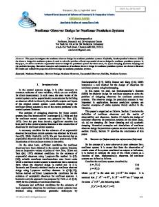
For this simulation, the tuning parameter 𝜌 is set to 10. The value of this parameter allows to adjust the convergence time of the observer given in Equation (27). Figures 1 and 2 show the states 𝑥1 (𝑡) and 𝑥2 (𝑡) and their estimated values 𝑥 ˆ1 (𝑡), 𝑥 ˆ2 (𝑡); it can be seen that after a brief period of time 𝑥 ˆ1 (𝑡) converge to 𝑥1 (𝑡). On

6. CONCLUSION In this work an observer for a class of delayed nonlinear triangular systems was presented. The time-delay is considered variable and it can be presented as a simple or multiple time-delay in the states or in the input of the system. The time-delay is supposed to be known and bounded. The main feature of the proposed observer with respect to others in the literature, is its simplicity. This is because (due to its particular structure) the system is treated in the original coordinates. Also, the observer gain is constant and does not require to solve any additional dynamical system. The observer is evaluated successfully through a simulation example. REFERENCES Fig. 1. The state 𝑥1 (solid line) and its estimated value 𝑥 ˆ1 (dashed line).

Fig. 2. The state 𝑥2 (solid line) and its estimated value 𝑥 ˆ2 (dashed line).

Fig. 3. The error estimation 𝑒1 and 𝑒2 . the other hand the time profile 𝑥2 (𝑡) and 𝑥 ˆ2 (𝑡) are quite similar. Figure 3 shows the errors estimations 𝑒1 and 𝑒2 , after a small time 𝑒1 and 𝑒2 converge to zero. It can be appreciated that 𝑥 ˆ2 (𝑡) converges very quickly to 𝑥2 (𝑡).

J.-P. Richard. Time-delay systems :an overview of some recent advances and open problems. Automatica, 39 :1667-1694, 2003. M. Darouach. Linear Functional Observers for Systems with Delays in State Variables. IEEE Trans. Automatic Control, 46(3) :491-496, 2001. A. Germani, C. Manes, et P. Pepe. A new approach to state observation of nonlinear systems with delayed output. IEEE Trans. Automatic Control, 47(1) :96-101, 2002. J.P. Gauthier, H. Hammouri, and S. Othman. A, A simple observer for nonlinear systems - application to bioreactors., IEEE Trans. on Aut. Control, 37:1992, pp 875-880. J.P. Gauthier and I.A.K. Kupka, Observability and observers for nonlinear systems, SIAM J. Control. Optim., 32:1994 pp 994-994. B. Targui, M. Farza, H. Hammouri,Observer design for a class of nonlinear systems, Applied Mathematics Letters, vol. 15, pp 709-720, 2002. B. Targui, H. Hammouri, M. Farza, Observer design for a class of multi-output nonlinear systems : application to a distillation column, 40th CDC (IEEE Conference on Decision and Control),pp 3352-3357, 2001. H. Hammouri, B. Targui and F. Armanet, High gain observer based on trianguler structure, Int. Journal on Robust and Nolinear Control., vol. 12, pp 497-518, 2002. M. Farza, M. M’Saad and L. Rossignol , Observer desgin for a class of MIMO nonlinear systems, Automatica, vol. 40, pp 135-143, 2004. S. Ibrir, Adaptive observers for time-delay nonlinear systems in triangular form Automatica, Volume 45, Issue 10, Pages 2392-2399, 2009. M. Hou, P. Zitek, and R. J. Patton, An observer Design for Linear Time-dealy Systems, IEEE Transcations on Automatic Control, 47, 121-125, 2002. Z. Wang, D. P. Goodall and K. J. Burnham, On designing observers for time-delay systems with nonlinear disturbances. International Journal of Control, 75(11), 803811, 2002.