Odometry and Calibration Methods for Multi-Castor ...

2008 IEEE International Conference on Robotics and Automation Pasadena, CA, USA, May 19-23, 2008

Odometry and Calibration Methods for Multi-Castor Vehicles James Doebbler, Jeremy J. Davis, John L. Junkins, and John Valasek Aerospace Engineering Department, Texas A&M University College Station, TX 77843, USA {james.doebbler, jeremy.davis, junkins, valasek}@tamu.edu

Abstract— We are developing a mobile robot capable of emulating general 6-degree-of-freedom spacecraft relative motion. The omni-directional base uses a trio of active split offset castor drive modules to provide smooth, holonomic, precise control of its motion. Encoders measure the rotations of the six wheels and the three castor pivots. We present a generic odometric algorithm using a least squares framework which is applicable to vehicles with two or more castors and apply it to our unique vehicle configuration. As the accuracy of odometry algorithms depends on the accuracy to which the model parameters are known, a method to perform calibration on the physical robot is needed. We present a geometric calibration method based solely on internal sensor measurements. We present a range of simulation results comparing our odometry results to other algorithms under various systematic and non-systematic errors. We evaluate the ability of our calibration method to accurately determine the true values of our system parameters. The odometry algorithm was also implemented and tested in hardware on our robotic platform. The results presented in the paper validate the calibration and odometry algorithms in both simulation and hardware.

I. I NTRODUCTION Multi-vehicle proximity operations of spacecraft, from formation flying to automated rendezvous and docking, represent an extremely active area of current research as industry moves toward smaller, cheaper satellites. Groundbased testing of the autonomous control algorithms for multiple vehicles with sensors or docking hardware in-theloop provides significant risk reduction for such missions. We are developing a relative motion emulator based on multiple mobile platforms, termed Relative Motion Vehicles (RMVs), consisting of an omni-directional base with a Stewart platform mounted atop [1]. The base provides large motions in 3-degrees-of-freedom (DOF), whereas the Stewart platform provides smaller motion in all 6-DOF to a high degree of precision, so it can be used to “clean-up” the less precise motion of the base. The mobile platform approach provides several distinct advantages over existing facilities like NRL’s Proximity Operations Testbed [2] and NASA’s Flight Robotics Facility [3]: 1) Allows for un-tethered circumnavigation of two or more vehicles. 2) Mobile nature enables testing or demonstration at any location with a large enough workspace. 3) Provides a low-cost alternative to larger installations while maintaining high fidelity. 4) Supports testing of non-spacecraft multi-vehicle systems, such as autonomous aerial refueling.

978-1-4244-1647-9/08/$25.00 ©2008 IEEE.

While Stewart platforms meeting the needs of this project are commercially available, the omni-directional base must meet motion requirements exceeding typical mobile robot designs. For instance, conventional robots have undesirable coupling between translation and rotation due to steering dynamics. We have designed an omni-directional base utilizing a trio of active split offset castors (ASOCs) to achieve the desired motion. Current methods of odometry focus primarily on a standard two-wheeled differentially-steered vehicle. The odometry equations for these drive types are well known and widely used. Borenstein presents a method called Internal Position Error Correction (IPEC), which uses a vehicle with two castors to achieve an order of magnitude improvement in odometry performance over a single-castored vehicle [4]. In this paper, we generalize and extend the ideas of IPEC to vehicles with two or more castors, with specific application to our three-castored ASOC vehicle. Critical to the odometry process is precise knowledge of many internal geometric parameters. Whereas multiple calibration methods exist for the standard two-wheeled robot, the process is much more difficult for multi-castored robots. We address the problem by providing a geometric solution to parameter determination using the robot’s internal sensors. This paper presents details of algorithms to perform calibration and odometry on an omni-directional mobile base for use in emulating on-orbit proximity operation dynamics. Drive train selection and design is discussed in Section II. Algorithmic details of both the odometry and calibration methods necessary to achieve the high precision positional knowledge through internal angle encoders are discussed in Section III, with simulation results being presented in Section IV. Results from testing these algorithms using a onethird scale prototype are discussed in Section V. Section VI presents conclusions and recommendations for future work. II. D ESIGN C ONFIGURATION This section overviews key aspects of the physical design of the RMVs and the associated design decisions. A. Defined Requirements True holonomic omni-directional motion of the base must be achieved with strict motion and sensing requirements as discussed in [1]. Since the errors in the base position can be corrected using the Stewart platform, the base control accuracy is an order of magnitude lower than the desired

2110

Authorized licensed use limited to: Texas A M University. Downloaded on July 02,2010 at 23:18:46 UTC from IEEE Xplore. Restrictions apply.

^

b2

c^ 2

c^ 1 θ

2

1

n^ 2

^

b1

ψ n^ 1

c^ 2 c^

1

Fig. 1.

Active Split Offset Castor (ASOC)

Base

c^

1

position knowledge. We set a target mass of 300 kg for the mobile base - an order of magnitude heavier than the Stewart platform - so that the motion of the Stewart platform and payload can be treated as a minor disturbance when controlling the RMV. Developing an omni-directional robot of such proportions with such stringent tracking and knowledge requirements results in a unique design configuration. B. Drive Mechanism The key design consideration of the mobile base is the drive configuration. In order to accurately model the dynamics of a spacecraft docking maneuver, the overall RMV must be able to accurately follow the desired trajectory. Several different drive mechanisms were considered for the mobile base, including individually steerable wheels, Mecanum wheels, and steerable offset castors [1]. We have adopted an attractive alternate drive method that uses drive modules consisting of a configuration known as an active split offset castor [5][6]. The ASOC design consists of two independently driven motors mounted along a common axis on a castor that is attached to the mobile base by a freely rotating vertical pivot. The axis of the wheels is offset in the horizontal plane from the pivot point in the direction perpendicular to the wheel axis. This creates a physical design such that any planar velocity of the pivot point can be achieved by driving the two independent wheels. The general concept is depicted in Fig. 1. A vehicle driven with at least two of these castors can achieve true holonomic motion with no steering dynamics, thus achieving the same advantages as the single offset castor while reducing the scrubbing torque. Though there are six motorized wheels, the total number of motors is the same as the steerable wheels considered previously. Unlike steerable wheels, however, all of the motors can be exactly the same, an advantage in terms of motor characterization, maintenance, and supportability. C. Drive Module Layout A minimum of three wheel modules are required for stability, and at least two of the castors must be powered. The third wheel module can be either passive or driven. We selected the option of having all three castor modules being driven and controlled, as it allows a more even distribution of motor torques between the motors throughout the envelope of

Pivot Castor

c^ 2

Wheel 3 Fig. 2.

Relative Motion Vehicle

allowable trajectories. The distribution of the three powered castors can be seen in Fig. 2. We define the locations of the pivots using polar coordinates (Ri , φi ) with respect to the body-fixed B-frame. Note that the choice of the location and orientation of the body-fixed frame is completely arbitrary. For simplicity, we designate the center of the three pivots as the origin of the B-frame and select castor 1 to lie along the bˆ 1 axis (φ1 = 0). D. Kinematics and Control We have developed the kinematics using a body-fixed B frame, that is fixed to the base of the robot and three castor-fixed Ci frames as seen in Fig. 2. The angle the B frame makes with the inertial N frame is denoted ψ , whereas the angle each castor makes with respect to the Bframe is denoted θi . By assuming no wheel slippage and by measuring the castor angles, the body-axis linear and angular velocities uniquely map into the six wheel velocities. Control is accomplished through a kinematics-based controller using feedback of wheel velocities and measurements of θi from angular encoders mounted on each pivot [1][7]. III. A LGORITHMS The overall system will incorporate a combination of “dead-reckoning”, or internal position feedback, and a periodic external inertial update. This section describes a method for highly accurate calibration as well as a multi-castor odometry algorithm for internal position measurement. A. Calibration Since odometry methods inherently rely on geometric paramters, pose estimates from odometry can only be as accurate as the calibration allows. Borenstein has developed a calibration method using the results of the University of Michigan Benchmark (UMBmark) test for a two-wheeled robot [8], and other researchers have put forth a variety of other methods improving on the UMBmark calibration for a differentially driven robot [9][10]. For any multi-castored vehicle, however, calibration methods are non-existent in

2111 Authorized licensed use limited to: Texas A M University. Downloaded on July 02,2010 at 23:18:46 UTC from IEEE Xplore. Restrictions apply.

about the pivot of the stationary castor in either a clockwise (CW) or counter-clockwise (CCW) manner. The angular distance traveled by each wheel, ci , is recorded, as is the angular distance through which the stationary castor pivot rotates, ∆θ . The path angle Γ can be calculated from the angles reported by the pivot encoders, γ , from the runs in both CW and CCW directions as follows: 180◦ − (γCCW − γCW ) (1) Γ= 2 We define θ⊥ to be the angle that should be measured by the castor encoder when the castor is aligned with the direction of travel in the CW maneuver. Note that θ⊥ is defined geometrically by the choice of the B-frame with respect to the pivots. Combined with the measured castor angles, γ , the pivot encoder bias, β , is found using:

castor direction r’c

d’1

rw1

α

Γ

rw2 direction of travel

d’2

D (measured) true castor direction θ

measured castor direction γ

rw1 Fig. 3.

∆θ

rc

β

d1

d2

rw2

Calibration set-up and definition of parameters

γCCW + γCW − 180◦ (2) − θ⊥ 2 Additionally, a simple geometric relationship provides rc : β=

the literature, and the calibration problem is an order of magnitude more challenging. As described in the previous section, each motor/wheel assembly is equipped with an incremental encoder to record wheel rotations, and each vertical pivot is equipped with an absolute encoder to measure castor angles. We have developed a geometric approach for calibrating our three castor mobile robot that relies entirely on these internal sensor measurements, though this method could be applied to any vehicle with more than one powered castor. We make only two assumptions about the configuration for this approach. First, the distance between any two castor pivots, D, is assumed to be known. This parameter is easily measured prior to attaching castors to the pivot shafts. Second, we assume that the two wheel axles on a given castor are colinear, something that can be assured if the wheel bearings on a castor are mounted with a single shaft passing through all of them. This second assumption is one implicitly assumed in all two-wheeled robot calibration methods. The parameters to be estimated are • • • •

rc - the length of the line perpendicular to the wheel axles passing through the pivot, rwi - the wheel radii, di - the distance from the wheels to the pivot along the axle, and β - the difference between the true castor angle θ , and the measured castor angle γ

as shown in Fig. 3. Note from the left side of the figure that an angular misalignment of the wheel axis of 90◦ − α can be transformed into a pivot angle misalignment β and a new set of rc and di parameters. The β term not only handles this angular misalignment of the wheels, but also compensates for any pivot encoder angle bias. The reference motion for calibration is simply to hold one of the castors stationary while applying a small constant voltage to the remaining wheels. By aligning the active castors in one direction or another, the robot will revolve

rc = D sin Γ

(3)

Both the CW and CCW runs provide information in the following form regarding the relationship between wheel radius, wheel base, and the measured quantities. ∆θCW (D cos Γ + d1 ) = cCW1 rw1 ∆θCW (D cos Γ − d2 ) = cCW2 rw2 ∆θCCW (D cos Γ − d1 ) = cCCW1 rw1 ∆θCCW (D cos Γ + d2 ) = cCCW2 rw2

(4) (5) (6) (7)

Solving these equations for rw produces: rwi =

2D cos Γ (∆θCCW ∆θCW ) ∆θCCW cCWi + ∆θCW cCCWi

(8)

And solving for d leaves the equation: di =

si D cos Γ (∆θCCW cCWi − ∆θCW cCCWi ) , ∆θCCW cCWi + ∆θCW cCCWi

s1 = 1, s2 = −1

(9) Thus, all parameters of a given castor can be estimated from a single run CW and CCW about a stationary castor. In our case, with three castors, executing rotations about all three castors provides two estimates for each castor’s parameters that we can average to provide improved accuracy. It is important to note that this procedure merely requires the active wheels to be commanded a voltage low enough that no wheel slippage occurs - no additional rigs or measuring apparatus are required. B. Odometry The internal encoders can be used to integrate the motion of the wheels to form an inertial position estimate, a process referred to as odometry. As with all dead-reckoning schemes, odometry is subject to accumulation of error, and estimates based on encoders must be updated with an external measurement or landmark recognition. Odometry is subject to both systematic errors, such as errors in wheel radii estimates,

2112 Authorized licensed use limited to: Texas A M University. Downloaded on July 02,2010 at 23:18:46 UTC from IEEE Xplore. Restrictions apply.

and non-systematic errors, such as floor irregularities, wheel slippage, or typical random measurement error. It is important to note that in odometry, unlike IMU integration, error accumulates as a function of distance traveled rather than as a function of time. Borenstein provides a detailed discussion of odometry methods and sources of error [11][12]. Of particular interest is the OmniMate Mobile Robot - an omni-directional platform that uses two powered split castors with additional free castors for stability. Using the Internal Position Error Correction (IPEC) algorithm he developed, Borenstein was able to reduce the dead-reckoning uncertainty of OmniMate by an order of magnitude compared to conventional wheeled robots [4]. This is intuitive, since each castor could provide its own inertial position estimate and with the relationship - angles and distance - between the two castors measured, the position of the vehicle is known with improved accuracy. This result applies to the mobile platform developed here with three independent castors, and should allow for further improvement on the 0.1% average accumulation error seen with OmniMate [8]. The IPEC algorithm is built on the premise that errors in heading angle lead to pose estimate errors that are orders of magnitude larger than the small translational errors introduced at a given update. IPEC utilizes each castor’s position estimate to compute the heading angle of the vehicle through the geometric relationship ¶ µ y2 − y1 (10) ψ = arctan x2 − x1

∆ψ , results in the following equations which are linear in the unknowns (∆xc , ∆yc , ∆ψ ):

where ψ is the heading angle of the vehicle and (xi , yi ) are the coordinates of the center of each castor. Whereas the heading angle of each castor could be computed independently, this use of each castors translational information - which suffers minimally from systematic and non-systematic errors over a single step - reduces heading estimate errors. This vehicle heading estimate is combined with the measured castor angles to update the heading estimate of each castor, and the position of the second castor is updated to be consistent with the pose of the first castor. The IPEC method can be applied to any two castors on our platform by using the positions of the pivot points rather than those of the castors in the above equations - a distinction unique to having an offset castor. We have developed a method based on the ideas of IPEC that can be used for more than two castors to take advantage of all information available. First, we note that the inertial position of a pivot (xi+ , y+ i ) at time t + relates to the inertial position of the center of the robot (xc+ , y+ c ) by the following relationship

      ∆xc       X = ∆yc ,Y =   ∆y 1   ∆ψ  ∆y2    .. .

xi+ = xc+ + Ri cos(ψ + + φi ), xi−

= xc− + Ri cos(ψ − + φi ),

+ + y+ i = yc + Ri sin(ψ + φi ) (11) − − yi = yc + Ri sin(ψ − + φi ) (12)

∆xi = ∆xc − ∆ψ Ri sin(ψ − + φi ) ∆yi = ∆yc + ∆ψ Ri cos(ψ − + φi )

(13) (14)

Standard odometry equations as given by Borenstein [11] are adapted to compensate for the offset of the pivot from the wheel axis to generate the (∆xi , ∆yi ) from the wheel encoder readings. Thus, as in IPEC, we utilize only the information regarding translational motion of each castor to inform our heading estimate rather than the heading information from each castor. Equations 13 and 14 can be used in a linear least squares algorithm employing n castors. The validity of the small angle assumption depends on the angular rate of the vehicle and position update frequency. In practice, the low complexity of this algorithm allows high update frequencies to ensure the validity of this assumption. Even a robot rotating at 90◦ /sec with position updates at 20 Hz would see a ∆ψ of less than 5◦ at each update step. When applying such algorithms to hardware, algorithmic complexity must be considered. Given a measurement model of Y = HX with all measurements weighted equally, the linear least squares solution is given by X = (H T H)−1 H T Y

(15)

where 





∆x1 ∆x2 .. .

 (16)

and, 

    H =    

1 0 −R1 sin(ψ − + φ1 ) 1 0 −R2 sin(ψ − + φ2 ) .. .. .. . . . 0 1 R1 cos(ψ − + φ1 ) 0 1 R2 cos(ψ − + φ2 ) .. .. .. . . .

         

(17)

Significant computational savings can be achieved by precomputing the required matrix inverse which takes the form  2  c − nd −bc nb 1  −bc b2 − nd nc  (H T H)−1 = n(b2 + c2 − nd) nb nc −n2 (18) where

where Ri and φi describe the position of the pivot with respect to the center of the robot. The corresponding relationship at t − is also shown. Subtracting these two equations and making a small angle assumption about the change in heading angle,

b = −n(my cos ψ − + mx sin ψ − ) c = n(mx cos ψ − − my sin ψ − )

(19) (20)

n

d

=

∑ R2i

i=1

2113 Authorized licensed use limited to: Texas A M University. Downloaded on July 02,2010 at 23:18:46 UTC from IEEE Xplore. Restrictions apply.

(21)

TABLE I M EAN PARAMETRIC ERRORS OVER 1000 Parameter rc rw d β

Uncalibrated 0.21% 2.07% 0.89% 7.98◦

TABLE II UMB MARK T EST S IMULATION R ESULTS

SIMULATIONS

Algorithm IPEC-1 CAST-1 CAST-0

Calibrated 0.09% 0.04% 0.04% 0.01◦

and mx and my are the x − y coordinates in the body frame describing the “center of mass” of the pivots with respect to the center of the vehicle. Note that defining the center of the robot to be the center of the three pivots results in b = c = 0, and Eq. 15 simplifies to   ∆xc X =  ∆yc  = ∆ψ   ∆xi 1 n   (22) ∆yi n ∑i=1 1 − − R (∆yi cos(ψ + φi ) − ∆xi sin(ψ + φi )) In this special case, the translation of the center of the base is simply the average of the motion measured by each castor. Just as in IPEC, the final, critical, step is to update the heading angle of each castor with the newly computed vehicle heading and the measured castor angles. It should be noted that in the case with more than two castors, the redundant information could be used to detect when a castor has been subjected to large non-systematic errors. Once detected, this invalid information could be disregarded from the final odometric position estimate in order to increase robustness to these errors. This extension is not the focus of this paper and is left for future study. IV. S IMULATION In order to test the validity of both algorithms, we performed simulations using 1000 different sets of randomly varied parameters. The mean errors of each parameter from the true value are listed as the uncalibrated values in Table I.

Uncalibrated Emax 394.6 mm 6.89% 394.1 mm 6.88% 311.0 mm 5.43%

Calibrated 71.7 mm 71.6 mm 39.0 mm

Emax 1.25% 1.25% 0.68%

computed, and the maximum of these two values provides a measure of the accuracy of the odometry, Emax . We simulated a robot based on the dimensions of our prototype traversing a 1.5 meter square with random parametric errors consistent with the measurement uncertainties of our uncalibrated prototype shown in Table I, with the exception of β , which we assumed to be zero. All encoder readings were produced with quantization errors and an update rate of 20 Hz. We simulated the UMBmark test on 1000 different sets of parameters and computed the average value of Emax over those runs for several different algorithms. We first implemented IPEC, considering only two castors, and then implemented our least squares solution using the same two castors as well as all three castors. We denote these combinations as IPEC-i and CAST-i, where i represents the castor not used. Following this notation, CAST-0 represents the solution with no castor excluded: the least squares solution using all three castors. Table II shows the results of the UMBmark test simulation using the uncalibrated parameters, including the error as a percent of distance traveled. The large numbers shown for the uncalibrated cases in Table II are a result of large parametric uncertainties - up to 4% in some cases - but this has no effect on the comparison of one algorithm to another. The two-castor least squares provides nearly the same solution as IPEC, whereas the three-castor solution shows a 20% improvement. After calibration, the odometry simulation was rerun with the calibrated parameters, and the pose estimation errors reduced by a factor of 5-8 as seen in the calibrated results of Table II. The three-castor least squares improves the estimate by almost a factor of 2 over either two-castor estimate. V. H ARDWARE - BASED I MPLEMENTATION

A. Calibration As discussed earlier, accurate calibration is required for the odometry to achieve the accuracies required for our system. To evaluate our approach, we ran 1000 different sets of parameters through the calibration algorithm. We compare the mean absolute error of the calibrated numbers over all 1000 runs to the mean parametric errors prior to calibration. Orders of magnitude improvement in the parameter estimates can be seen in Table I. B. Odometry The UMBmark test consists of the robot traversing a square both clockwise and counterclockwise five times and measuring the position estimate error at the end of each circuit [8]. The magnitude of the average position error for both clockwise (rCW ) and counterclockwise (rCCW ) is

In this section, we discuss a one-third scale prototype that was used to demonstrate design feasibility and for use in testing and development of data fusion techniques, control laws, and a dynamics model of the full-scale platform. The actuator and sensor configurations of the full-scale platform were implemented on the prototype to accurately evaluate state estimation and control methods. The prototype presented here possesses all of the required sensors, but at lower precisions than the full-size mobile platform. The prototype has optical encoders on the wheels and on the pivots, so that data can be used in feedback control laws just like the full scale implementation. The wheel encoders can measure in increments of 0.3◦ , whereas the pivot encoders can measure in increments of 0.07◦ . Fig. 4 shows a picture of the one-third scale prototype.

2114 Authorized licensed use limited to: Texas A M University. Downloaded on July 02,2010 at 23:18:46 UTC from IEEE Xplore. Restrictions apply.

TABLE III P ROTOTYPE TEST RESULTS Algorithm IPEC-1 IPEC-2 IPEC-3 CAST-1 CAST-2 CAST-3 CAST-0

540 511 458 544 459 432 191

Emax mm mm mm mm mm mm mm

9.5% 9.0% 8.0% 9.5% 8.0% 7.6% 3.3%

VI. C ONCLUSIONS AND F UTURE W ORK

Fig. 4.

Algorithms for multi-castor calibration and odometry have been presented. Simulation results verify both approaches when compared to the true parameters and IPEC, and the tests in hardware using our prototype further validate the algorithms. The next step is to test these algorithms on another platform and implement the least squares odometry algorithm as realtime feedback for control purposes. We are currently designing the full-scale version of our prototype to complete this testing.

Prototype mobile base with joystick controller

0.5 0.4 0.3

Error in y (m)

0.2

R EFERENCES

0.1 0 −0.1

IPEC−1 IPEC−2 IPEC−3 CAST−1 CAST−2 CAST−3 CAST−0

CCW

−0.2 −0.3 CW

−0.4 −0.5

−0.4

−0.2

0 Error in x (m)

0.2

0.4

0.6

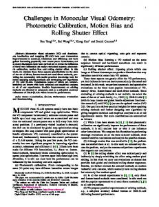
Fig. 5. Results of UMBMark test using prototype. IPEC-i and CAST-i refer to the ith castor being excluded. CAST-0 uses all 3 castors

The one-third scale hardware platform has been completed and can be controlled using either a joystick or pre-defined trajectories which it follows open-loop. We present here the results of a slightly modified UMBmark test using the prototype to evaluate the wheel odometry position estimation algorithms discussed earlier. To complete this test, the data was collected for four runs in each direction along a 1.5 m square and then run through each of the algorithms offline. Fig. 5 shows the final errors for each run for each algorithm, and Table III shows the average error, Emax . We show the results for IPEC by using only two of the three castors at a time, in all three combinations since parametric errors lead to different results for different combinations of castors. We also present our corresponding least squares solutions. As in the simulation, the two-castor least squares results very nearly match the IPEC results, and the three castor result (CAST-0) provides the best solution. As in the odometry simulation, these errors are large overall and have meaning only for comparisons of algorithms until the calibration methods have been employed.

[1] J. Davis, J. Doebbler, K. Daugherty, J. Junkins, and J. Valasek, “Aerospace Vehicle Motion Emulation Using Omni-directional Mobile Platform,” in Proceedings of AIAA Guidance, Navigation, and Control Conference, Hilton Head, SC, Aug 2007. [2] G. Creamer, F. Pipitone, C. Gilbreath, D. Bird, , and S. Hollander, “NRL Technologies for Autonomous Inter-Spacecraft Rendezvous and Proximity Operations,” in Proceedings of the John L. Junkins Astrodynamics Symposium, AAS/AIAA Space Flight Mechanics Meeting, College Station, Texas, May 2003, paper AAS 03-272. [3] F. D. Roe, D. W. Mitchell, B. M. Linner, and D. L. Kelley, “Simulation Techniques for Avionics Systems - An Introduction to a World Class Facility,” in Proceedings of the AIAA Flight Simulation Technologies Conference, San Diego, California, July 1996, paper 96-3535. [4] J. Borenstein, “Experimental Results from Internal Odometry Error Correction with the OmniMate Mobile Robot,” IEEE Transactions on Robotics and Automation, vol. 14, no. 6, Dec. 1998. [5] H. Yu, M. Spenko, and S. Dubowsky, “Omni-Directional Mobility Using Active Split Offset Castors,” ASME Journal of Mechanical Design, vol. 126, no. 5, pp. 822–829, Sept. 2004. [6] M. Spenko, H. Yu, and S. Dubowsky, “Analysis and Design of an Omnidirectional Platform for Operation on Non-Ideal Floors,” in Proceedings of IEEE International Conference on Robotics and Automation, vol. 1, Washington DC, May 2002, pp. 726–731. [7] X. Bai, J. J. Davis, J. Doebbler, J. Turner, and J. L. Junkins, “Dynamics, Control and Simulation of a Mobile Robotics System for 6-DOF Motion Emulation,” in World Congress on Engineering and Computer Science, San Francisco, CA, Oct 2007. [8] J. Borenstein and L. Feng, “UMBmark: A Method for Measuring, Comparing, and Correcting Dead-reckoning Errors in Mobile Robots,” University of Michigan, Ann Arbor, Michigan, Tech. Rep. UMMEAM-94-22, Dec. 1994. [9] T. Abbas, M. Arif, and W. Ahmed, “Measurement and Correction of Systematic Odometry Errors Caused by Kinematics Imperfections in Mobile Robots,” in SICS-ICASE International Joint Conference, Bexco, Busan, Korea, October 2006. [10] P. R. Kedrowski, C. F. Reinholtz, and D. C. Conner, “Optimized parametric calibration of autonomous vehicles,” in Proceedings of the SPIE The International Society for Optical Engineering, Newton, MA, Oct 2001. [11] J. Borenstein, H. Everett, and L. Feng, Navigating Mobile Robots: Sensors and Techniques. Wellesley, MA: AK Peters Ltd, 1996. [12] J. Borenstein, H. Everett, L. Feng, and D. Wehe, “Mobile Robot Positioning: Sensors and Techniques,” Journal of Robotic Systems, vol. 14, no. 4, pp. 231–249, 1997.

2115 Authorized licensed use limited to: Texas A M University. Downloaded on July 02,2010 at 23:18:46 UTC from IEEE Xplore. Restrictions apply.