On Combining Expertise in Dynamic Linear Models Jesus Palomo, David Rios Insua and Fabrizio Ruggeri Technical Report #2005-6 July 27, 2005 This material was based upon work supported by the National Science Foundation under Agreement No. DMS-0112069. Any opinions, findings, and conclusions or recommendations expressed in this material are those of the author(s) and do not necessarily reflect the views of the National Science Foundation.
Statistical and Applied Mathematical Sciences Institute PO Box 14006 Research Triangle Park, NC 27709-4006 www.samsi.info
On combining expertise in Dynamic Linear Models Jesus Palomo, David Rios Insua and Fabrizio Ruggeri SAMSI and Duke University, Universidad Rey Juan Carlos and CNR-IMATI Durham, USA, Madrid, Spain, Milano, Italy
[email protected],
[email protected],
[email protected]
Abstract. We consider different models combining opinions of two experts given at specific time points when forecasting with dynamic models. We describe a Bayesian approach for inference and prediction in such situations, using both historical data and current expert’s opinions. We consider cooperation cases in which experts’ opinions are merged into a class of priors or an expert provides information to the other one, and compare these cases with the non-cooperative, independent one. The former case leads to robust Bayesian analyses, whereas in the latter the expert’s input is treated as information used to improve upon the basic model and learn about the expert’s quality, in the sense of ability in forecasting. Our approach is motivated by the need of companies to forecast project costs in bidding processes. Keywords: Dynamic model, Project costing, Expert’s opinion, Bayesian forecasting, Bayesian robustness.
1
Introduction
We consider the case of two experts who are faced with the problem of formulating opinions on a series of similar events at different times (e.g. bidding in off-shore oil plant auctions). The cost structure is evolving over time and decisions are to be taken combining both historical data and experts’ opinions. Dynamic linear models (DLM’s) are typical choices to address this problem and the Bayesian approach is the natural framework to combine past evidence and expertise. We suppose the two experts (but their number could be larger) have different knowledge and we explore different ways to combine their expertise. We suppose the experts have to report decisions based on their opinions to the top management of a company. We explore three cases: • the experts act independently and each of them reports his/her own decision; • the experts combine their opinions into a class and consider consequences of such action; • one expert expresses his/her own opinion and updates it using the other expert’s opinion as data. The first case is treated with the well-known methods in the Bayesian analysis of dynamic linear models; see (West and Harrison 1997) for a thorough review. The second case is treated with methods from Bayesian robustness; see (Rios Insua and Ruggeri 2000) for a review. The third case is an example of a general model developed in (Palomo et al. 2004). We are here exploring also issues such as the experts’s quality and what happens when ignoring the information they provide. Some suggestions on these issues may be seen in (Spiegelhalter et al. 1994), for when to ignore expert’s opinions, and (Clemen and Winkler 1999), when more than one expert opinion is available. The paper is structured as follows: in Section 2, we illustrate the project which has lead us to consider the problem of combining opinions in DLM’s. Section 3 reviews the key issues in robust Bayesian analysis. In Section 4, we introduce the basic DLM and illustrate the case of independent experts. In Section 5, we apply methods from Bayesian robustness to the case of opinions joined into classes of priors. Section 6 illustrates a DLM in which an expert uses the other expert’s opinion to update his/her own. Section 7 illustrates the proposed methods in an example. We finish with some discussion.
2
Project description
The paper stems from a consulting project in which a framework to cope with the problem of bid formulation in off-shore oil plant auctions was required. Project cost forecasting is an essential step in project management and is becoming increasingly involved because of financial uncertainties, sometimes caused by the use of innovative technologies. Several project management techniques have been proposed, see (Turner 1993) for a review. However, in the current economy where auctions have become a daily activity with which companies must deal, these traditional techniques are no longer sufficient. In this competitive environment, project cost
forecasting becomes especially crucial, since an accurate estimation of the project cost distribution allows bidders to prepare better bids, in terms of expected profits, while decreasing the probability of undercapitalization. In other words, auctions have increased the project’s uncertainties and have caused that a bad estimation of costs may lead a bidder to either loose the auction, or win it with a bid lower than the actual cost. Quite frequently, project costing techniques appeal to heuristics, with relatively few statistical methods being applied and, in general, do not allow to deal with all the uncertainties, neither to handle expert’s opinion, which may be essential when handling multi-component projects that span many professional areas in which the proposal manager (PM) will not be skilled. One example is the Activity-Based Costing (ABC) technique, see (Alan 1995) or (Raz and Elnathan 1998), which is used profusely in large scale industries to improve operational performance by providing product cost estimations. Although there is a large number of papers dealing with the design and implementation of the ABC technique, see e.g. (Berliner and Brimson 1988), (David and Robert 1995), or (Booth 1996), there is no procedure to account for the uncertainty in the cost estimations of each project’s activity. Therefore, since several benefits and important insights could be obtained by applying modelling uncertainty to activity costs, see (Garvey 2000) for a review, (Palomo et al. 2004) addressed the problem of finding the project total cost distribution through aggregation of the cost distributions of all project activities. Combining ideas on expert modelling, as e.g. in (Campodonico and Singpurwalla 1995), and of dynamic model, as e.g. in (West and Harrison 1997), (Palomo et al. 2004) proposed a Bayesian approach using a formal framework to incorporate historical data and expert’s opinions in a dynamic cost forecasting process. In the current paper we consider the cost of one project activity and we suppose two people are involved in forecasting its cost. The proposal manager (PM) is an expert on business matters, with scarce knowledge on the project activity but with a global view on the project and the economical/political/social situation (and its influence on costs) of the environment in which the plant is planned. The unit manager (UM) has a deeper technical knowledge on that particular project activity but a scarce knowledge on the whole project and the external conditions under which the plant should be built. Therefore, the two sources of knowledge are different and we propose different methods of combining them, whereas (Palomo et al. 2004) considered only the case in which the the PM had beliefs about the uncertain cost component ci at time i, and he asked for an expert’s forecast ti about it. Using this new information, the PM could update his beliefs to ci |ti and assess the expert’s forecasting quality along different projects.
3
Bayesian robustness
As criticized by non-Bayesians and recognized by Bayesians, the choice of a prior distribution is a critical aspect of the Bayesian approach since different choices could lead to very different answers. Although the elicitation of a prior should be performed as carefully as possible, uncertainty in specifying prior beliefs cannot be avoided, in general. Robust Bayesian Analysis is concerned with the sensitivity of the results of a Bayesian analysis to the inputs for the analysis, mostly in replacing a single prior distribution by a class of priors, and developing methods of computing the range of the ensuing answers as the prior varies over the class. Interest naturally expands into study of robustness with respect to the likelihood and loss function as well, with the aim of having a general approach to sensitivity towards all the ingredients of the Bayesian paradigm (model/prior/loss). The usual practical motivation underlying robust Bayesian analysis is the difficulty in assessing the prior distribution. A common elicitation technique about continuous random variables is to discretize their range Θ and to assess the probabilities of the resulting sets. One actually ends up only with some constraints on these probabilities. This is often phrased in terms of having bounds on the quantiles of the distribution. A related idea is having bounds on the distribution function corresponding to the random variable. Once again, qualitative constraints, such as unimodality, might also be added. Perhaps most common for a continuous random variable is to assess a parameterized prior, say a conjugate prior, and place constraints on the parameters of the prior; while this can be a valuable analysis, it does not serve to indicate robustness with respect to the specified form of the prior. Similar concerns apply to the other elements (likelihood and loss function) considered in a Bayesian analysis. The main goal of Bayesian robustness is to quantify and interpret the uncertainty induced by partial knowledge of one (or more) of the three elements in the analysis. Also, ways to reduce the uncertainty are studied and applied until, hopefully, robustness is achieved. As an example, suppose the quantity of interest is the posterior mean; the likelihood is considered to be known, but the prior distribution is known only to lie in a given class. The choice of the class is very important, it should have some desirable, but competing, properties • computation of robustness measures should be as easy as possible;
• all reasonable priors should be in the class and unreasonable ones (e.g. discrete distributions in many problems) should not; • class should be easily specified from elicited prior information. The uncertainty might be quantified by specifying the range, i.e. the difference between upper and lower bounds on the quantity of interest, spanned by the posterior mean, as the prior varies over the class. One must appropriately interpret this measure; for instance, one might say that the range is “small” if it spans less than 1/4 of a posterior standard deviation (suitably chosen from the range of possible posterior standard deviations). If the range is small, robustness is asserted, and the analysis would be deemed to be satisfactory. If, however, the range is not small, then some way must be found to reduce the uncertainty; narrowing the class of priors or obtaining additional data would be ideal. There are three main approaches to Bayesian robustness. The first is the informal approach, in which a few priors are considered and the corresponding posterior means are compared. The approach is appealing because of its simplicity and can help, but it can easily “miss” priors that are compatible with the actually elicited prior knowledge and yet which would yield very different posterior means. The second approach, called global robustness, considers the class of all priors compatible with the elicited prior information, and computes the range of the posterior mean as the prior varies over the class. This range is typically found by determining the “extremal” priors in the class that yield the maximum and minimum posterior means. Such computations can become cumbersome in multidimensional problems. The third approach, called local robustness, is interested in the rate of change in inferences, with respect to changes in the prior, and uses differential techniques to evaluate the rate. A general review of literature on Bayesian robustness is given in (Rios Insua and Ruggeri 2000). In this paper we consider both informal and global robustness. The former will be considered in Section 4 where effects of two priors will be considered and compared; the latter will be performed in Section 5 where the expert’s opinions will be joined in a class of priors.
4
Independent DLM’s
We suppose that the two experts are independent of each other. In this case a DLM describes their beliefs: 0
ci |θi ∼ N (Fi θi , Vi ) θi |θi−1 ∼ N (Gi θi−1 , Wi ) θ0 ∼ N (m0 , ∆0 )
(1)
For each time i, the model is characterized by the tuple {Fi , Gi , Vi , Wi }, with Fi a known (n x 1) matrix, Gi a known (n x n) matrix, Wi a known (n x n) variance matrix, and Vi is a known scalar variance. As illustrated in (West and Harrison 1997), the forecast on the cost ci follows from the standard DLM equations, i.e. π(ci ) ∼ N (fi , qi ), where 0
fi
= Fi Gi mi−1
qi
= Fi Riθ Fi + Vi
0
0
Riθ = Gi ∆i−1 Gi + Wi mi = Gi mi−1 + Aθi eθi Riθ
∆i = Aθi = eθi
(2)
0 − Aθi qi Aθi Riθ Fi q1i
= c˜i − fi
When the actual value c˜i arrives, the posterior on θi is obtained following standard DLM computations, see (West and Harrison 1997), π(θi |˜ ci ) ∼ N (mi , ∆i ), with mi , ∆i as before. The two experts can specify their own parameters and, once the values (˜ c1 , . . . , c˜n ) have been observed, comparison of forecasting and posterior distributions is quite straightforward since the distributions involved are normal ones.
We will show an example of comparison in Section 7.
5
Classes of priors in DLM
Experts may agree on a class of DLM’s or priors as representative of their joint belief. The simple way is to consider classes of priors on θ0 in the DLM (1). The simple class of priors is the one containing the two priors specified by the experts. Starting from them, the forecast distributions and the posterior estimators can be compared, performing an informal robustness check. A slightly wider class consider all the priors with parameters within a specified interval. Usually, the range of the posterior quantity of interest is achieved at endpoints of the interval. Ranges of other quantities in (1), e.g. F (when it is a scalar), can be easily considered. Despite of the plethora of papers published, specially in the 90’s, on Bayesian robustness, the application of these methods to DLM’s is rather scarce. In this paper, we do not plan to pursue a systematic analysis of robustness in DLM but we just want raise the awareness of the importance, although neglected, of robust studies in DLM. We will illustrate the robust Bayesian approach with an example in Section 7.
6
DLM with expert’s opinion
We suppose now an expert (the PM in our consulting project) uses a DLM for his basic forecasts and the other expert (the UM) provides point forecasts. The PM does not know exactly how the UM produces these estimates, but he assumes that the UM aims at being accurate. He tries to learn the UM’s forecasting quality for later periods and, hopefully, obtain a more informative forecasting distribution combining his model prediction with the UM’s opinion.
6.1
Formulation
The case we consider is described by the influence diagram in Figure 1. The PM is interested in forecasting the quantity ci at time i, both before and after having heard the UM’s opinion ti . We assume that the evolution of the ci ’s is appropriately described by a linear state-space model with state variable θi , which includes all unobservable factors affecting ci , like the economy, actual demand,. . . An accuracy parameter ai measures, somehow, the expert’s ability. We shall assume that ai = ti − ci is a bias, which follows an autoregressive process. Note that we are essentially combining three standard models, as illustrated in Figure 1. Block I describes the linear state-space model we use; block II describes a standard error model; block III describes a timevarying autoregressive model for the evolution of biases. Nonlinearity in Block I has been considered in the general model developed in (Palomo et al. 2004), and applied to a neural network example.
6.2
Inference and Prediction
As previously mentioned, the key issue is the prediction of ci , both before and after ti is heard. At any instant i, before any forecasting task takes place, we assume the PM has distributions for the variables βi and θi , which summarize all available information. For simplicity, we shall write them π(βi ), π(θi ), dropping any dependence from previously observed values c˜i−1 , t˜i−1 (and a ˜i−1 ). Specifically, the information processing is based on the following joint distribution π(ci , θi , ai , ti , βi ) = π(θi )π(ci |θi )π(ti |ci , ai )π(ai |βi )π(βi ) At each time i, we start with the distributions π(βi ) and π(θi ), and those given by the error model, the linear dynamic model and the autoregressive model. Before observing ti , the PM may provide a forecast for ci , based on π(ci ). Once he hears t˜i , he provides a forecast, based on π(ci |t˜i ). Then he observes c˜i , and a ˜i = t˜i − c˜i is found out. Finally, he obtains the priors π(βi+1 ) and π(θi+1 ) for the next period. The general model is described in (Palomo et al. 2004). Here we consider an important case in which computations may
Figure 1. Influence diagram for the dynamic model with expert input
be done analytically. Let θi evolve as a DLM, with the following distributional assumptions 0 ci |θi ∼ N (Fi θi , Vi ) I Linear state-space model θ |θ ∼ N (Gi θi−1 , Wi ) i i−1 θ0 ∼ N (m0 , ∆0 ) II Standard error model
©
ti |ci , ai ∼ N (ci + ai , Γi )
ai |βi ∼ N (βi ai−1 , Σi ) III Standard autoregressive model βi |βi−1 ∼ N (βi−1 , Ωi ) β0 ∼ N (µ0 , Λ0 ) For each time i, the model is characterized by the tuple {Fi , Gi , Vi , Wi , Γi , Σi , Ωi }, with Fi a known (n x 1) matrix, Gi a known (n x n) matrix, Wi a known (n x n) variance matrix, and Vi , Γi , Σi , Ωi are known scalar variances. The previous forecasting iterative process can be described analytically as follows • Before hearing ti , forecast with the standard DLM equations from π(ci ) ∼ N (fi , qi ), as in (2) when independent experts were considered. • After hearing t˜i , forecast from π(ci |t˜i ) ∼ N (fi∗ , qi∗ ), where 0
fi∗ = Fi δi Gi mi−1 +
Vi (t˜i −˜ ai−1 µi−1 ) Γi +Vi
Vi2 ξi2 0 (Γi +Vi )2 (Vi ξi −Fi φi Fi Γ2i )
qi∗
=
δi
i +Vi ) ∗ = φi [Riθ ]−1 Γi (Γ qi Vi ξi i h 0 −1 = [Riθ ]−1 + Fi VΓi 2ξi Fi
with
φi
i
ξi = Vi (Riβ a ˜2i−1 + Σi ) + Γi (Γi + Vi ) Riβ
= Ωi + Λi−1
Observe the correction from fi to fi∗ in the above results. Note that, when θi is unidimensional, we can write the predictive mean as · ¸ Vi ξi Vi Γi ∗ fi + fi = (t˜i − a ˜i−1 µi−1 ) −1 θ 0 2 Γi + Vi Ri [Vi ξi φi − Fi Γi Fi ] Γ i + Vi where fi is corrected by a factor which depends on the variances of the predictive distributions of ci and ai . The second term considers the expert’s opinion corrected by a forecast of his own bias (t˜i − ai−1 µi−1 ) i . times the factor ΓiV+V i It is also interesting to consider several extreme cases. When the expert is a clairvoyant (ai = 0, Γi = 0, ∀i = 1, . . . , n), we have δi = 0, so fi∗ = t˜i and qi∗ = Σi : the predictive density is centered on the expert’s opinion t˜i , with variance equal to the expert’s bias variance. When the expert is very unreliable (Γi → ∞), q∗ Vi2 i we have fi∗ → 2VVi −q fi = Vii fi and qi∗ → 2Vi −q . Notice that, in this case, we ’forget’ the expert’s i i opinion t˜i and his quality parameters (ai ,Σi ,Γi ). • When the actual value c˜i arrives, the posteriors are obtained following standard DLM computations, see (West and Harrison 1997), π(θi |˜ ci ) ∼ N (mi , ∆i ), with mi , ∆i as before. π(βi |˜ ai ) ∼ N (µi , Λi ) = µi−1 + Aβi eβi
µi Λi
=
Aβi
=
eβi
Riβ Σi β 2 Ri a ˜i−1 +Σi Riβ a ˜i−1
Riβ a ˜2i−1 +Σi
=a ˜i − µi−1 a ˜i−1
• The priors for the next period are obtained, using standard DLM computations, as follows π(θi+1 |˜ ci )
θ ∼ N (Gi+1 mi , Ri+1 )
β π(ai+1 |˜ ai ) ∼ N (µi a ˜i , Ri+1 a ˜2i + Σi+1 )
7
An example in project cost forecasting
(Palomo et al. 2004) addressed the estimation of a project total cost using data from a case study on ABC technique in (Gunasekaran and Singh 1999). The study is focused on estimating the total production cost of machines for the photo framing industry. Here we illustrate our methods just for the assembly activity which involves 82 units. The quantity of interest is the cost per unit. We show now one iteration of the estimation process in the three cases we have illustrated in the previous Sections.
7.1
Independent DLM’s
We suppose that the two experts act independently. We specify for each of them a DLM (1). Since all the distributions involved in the DLM are, at each stage, normal ones, then we consider, without loss of generality, the first cost c1 . We suppose that the first expert specifies c1 |θ1 ∼ N (θ1 , 1) θ1 |θ0 ∼ N (θ0 , 0.05) θ0 ∼ N (11, 0.05). With these assumptions, it follows that the forecast distribution is π(c1 ) ∼ N (11, 1.1),
whereas the posterior distribution becomes π(θi |˜ c1 ) ∼ N (10.98, 0.091) when the actual cost c˜1 = 10.81 is observed. The second expert specifies a model which starts with (possible) larger values due to a larger m0 but it should shrink over time since F = 0.9. His DLM is c1 |θ1 ∼ N (0.9θ1 , 1) θ1 |θ0 ∼ N (θ0 , 0.05) θ0 ∼ N (12, 0.05), so that he gets π(c1 ) ∼ N (10.8, 1.85) π(θ1 |˜ c1 ) ∼ N (11.39, 2.04). It is worth mentioning that in both cases the posterior mean of θ1 |˜ c1 lies between c˜1 and m0 . The change in F affects the variances of the distribution of the second expert, more than the change in m0 (which, alone, would have not changed the variances with respect to the first expert).
7.2
Classes of priors in DLM
Suppose the two experts agree in considering the class of DLM’s given by c1 |θ1 ∼ N (θ1 , 1) θ1 |θ0 ∼ N (θ0 , 0.05) θ0 ∼ N (m0 , 0.05), with m0 ∈ [11, 12], i.e. within the two prior opinions of the experts. In this case, it can be shown that π(θ1 |˜ c1 ) ∼ N (K, 0.091), 10.98 ≤ K ≤ 11.89.
7.3
DLM with expert’s opinion
Following the model presented in Section 6, the first expert (PM) obtains ci |θi ∼ N (θi , 1) θi |θi−1 ∼ N (θi−1 , 0.05) θi−1 ∼ N (11, 0.05) t1 |ci , ai ∼ N (ci + ai , 1) ai |βi ∼ N (−5βi , 0.1) βi |βi−1 ∼ N (βi−1 , 0.1) βi−1
∼ N (1, 0.1)
and the expert’s error in the previous forecast for ci was, say, a ˜i−1 = −1. As for the independent model, we obtain the same forecast before asking any expert’s opinion, i.e. π(ci ) ∼ N (11, 1.1). Then, we can obtain a point estimate from the expert UM, say, t˜i = 12, and, hopefully, a more accurate forecast distribution is obtained π(ci |t˜i ) ∼ N (11.13, 0.6). Note that with our approach, the proposal manager obtains:
• posterior information of the costs for future products or updates of the current one through a dynamic process. Following the detailed process for ci , when the actual cost c˜i = 10.81 arrives, the posteriors are obtained as follows: π(θi |˜ ci ) ∼ N (10.98, 0.091) π(βi |˜ ai ) ∼ N (−0.46, 0.067) where a ˜i = t˜i − c˜i = 1.19. For future products, we shall start with the following prior for assembly cost π(θi+1 |˜ ci ) ∼ N (10.98, 0.141) • learn about the expert’s quality for future elicitations which, in the case of the assembly unit manager, has the following prior for the bias π(ai+1 |˜ ai ) ∼ N (−0.55, 0.34)
8
Discussion
Although we have focused on project cost forecasting, the dynamic linear models combining different sources of expertise can be applied in many other fields. In the same company where the current project started, the same procedure could be used for time forecasting, which is a very relevant activity too. Currently, shorter delivery times are a very key issue in assigning subcontracts, and the control of the delivery time by the company is crucial to meet the final deadline signed with the auctioneer. These models can find applications in electronic democracy as a decision support tool since they relate opinions from different experts and different scenarios could be explored, specially when new evidence is available at some time points and the quantity of interest (the cost throughout the paper) evolves dynamically. Different level of cooperations between the experts are modelled in the previous Sections and they are suitable for a variety of practical situations. As mentioned before, robustness has been scarcely studied in DLM, probably because computations in more general DLM are more complex than what we showed here and robustness studies would become cumbersome. Even more difficult, although worthwhile, robustness analysis could be performed in the more general model by (Palomo et al. 2004).
Acknowledgments The research of J. Palomo was performed while he was working at the Statistics and Decision Sciences Group at Universidad Rey Juan Carlos, and visiting CNR-IMATI and SAMSI. This work was partially supported by grants from CICYT, CAM, URJC and the DMR Foundation at the Decision Engineering Lab. Also by fundings under the European Comission’s Fifth Framework ’Growth Programme’ via Thematic Network “Pro-ENBIS”, contract reference G6RT-CT-2001-05059. Research Programme CNR-MIUR on “Metodi e sistemi di supporto alle decisioni” Legge 95/95. The authors thank Enrico Cagno, Franco Caron, Mauro Mancini (Politecnico di Milano), Livio Colombo (Snamprogetti) for their helpful comments.
References Alan, W. (1995), “ABC: A Pilot Approach,” Management Accounting, 50–55. Berliner, C. and Brimson, J. (1988), Cost Management for Today’s Advanced Manufacturing -The CAM-I Conceptual Design, Harvard Business School. Booth, R. (1996), “Manifesto For ABC,” Management Accounting, 32–34. Campodonico, S. and Singpurwalla, N. (1995), “Inference and Predictions From Poisson Point Processes Incorporating Expert Knowledge,” Journal of the American Statistical Association, 90, 220–226. Clemen, R. and Winkler, R. (1999), “Combining Probability Distributions From Experts in Risk Analysis,” Risk Analysis, 19. David, E. and Robert, J. (1995), “Departmental Activity Based Management,” Management Accounting, 27– 30.
Garvey, P. (2000), Probability Methods for Cost Uncertainty Analysis: A systems engineering perspective, Marcel Dekker, New York, NY. Gunasekaran, A. and Singh, D. (1999), “Design of activity-based costing in a small company: a case study,” Computers and Industrial Engineering, 413–416. Palomo, J., Rios Insua, D., and Ruggeri, F. (2004), “Dynamic models with expert input with applications to Project Cost Forecasting,” Technical Report, CNR-IMATI, Milano, Italy. Raz, T., and Elnathan, D. (1998), “Activity Based Costing for Projects,” International Journal of Project Management, 61–67. Rios Insua, D., and Ruggeri, F. (eds.) (2000), Robust Bayesian Analysis, Springer-Verlag, New York. Spiegelhalter, D., Harris, N., Bull, K., and Franklin, R. (1994), “Empirical Evaluation of Prior Beliefs About Frequencies: Methodology and a Case Study in Congenital Heart Disease,” Journal of the American Statistical Association, 89, 435–443. Turner, J. (1993), The Handbook of Project-Based Management: Improving the Processes for Achieving Strategic Objectives, McGraw-Hill, New York. West, M. and Harrison, J. (1997), Bayesian Forecasting and Dynamic Models, 2nd ed, Springer-Verlag, New York..