On Deep Generative Models with Applications to Recognition Marc’Aurelio Ranzato∗ Joshua Susskind† ∗ Department of Computer Science University of Toronto
Volodymyr Mnih∗ Geoffrey Hinton∗ † Institute for Neural Computation University of California, San Diego
ranzato,vmnih,
[email protected]
[email protected]
Abstract The most popular way to use probabilistic models in vision is first to extract some descriptors of small image patches or object parts using well-engineered features, and then to use statistical learning tools to model the dependencies among these features and eventual labels. Learning probabilistic models directly on the raw pixel values has proved to be much more difficult and is typically only used for regularizing discriminative methods. In this work, we use one of the best, pixel-level, generative models of natural images – a gated MRF – as the lowest level of a deep belief network (DBN) that has several hidden layers. We show that the resulting DBN is very good at coping with occlusion when predicting expression categories from face images, and it can produce features that perform comparably to SIFT descriptors for discriminating different types of scene. The generative ability of the model also makes it easy to see what information is captured and what is lost at each level of representation.
Figure 1. Outline of a deep generative model composed of three layers. The input is a high-resolution image (or a large patch). The first layer applies filters that tile the image with different offsets (squares of different color are filters with different parameters). The filters of this layer are learned on natural images. Afterwards, a second layer is added. This uses as input the expectation of the first layer latent variables. This layer is trained to fit the distribution of its input. The procedure is repeated again for the third layer (and as many as desired). Because of the tiling, the spatial resolution is greatly reduced at each layer, while each latent variable increases its receptive field size as we go up in the hierarchy. After training, inference of the top level representation is well approximated by propagating the expectation of the latent variables given their input starting from the input image (see dashed arrows), which is efficient since their distribution is factorial. Generation is performed by first sampling from the top layer, and then using the conditional over the input at each layer (starting from the top layer) to back-project the samples in image space (see continuous line arrows). Except at the first layer, all other latent variables are binary. Generation can be used to restore images and cope with occlusion. The latent variables can be used as features for a subsequent discriminative classifier trained to recognize objects.
1. Introduction and Previous Work Over the past few years most of the research on object and scene recognition has converged towards a particular paradigm. Most methods [11] start by applying some wellengineered features, like SIFT [15], HoG [4], SURF [1], or PHoG [2], to describe patches of the image, and then they aggregate these features at different spatial resolutions and on different parts of the image to produce a feature vector which is subsequently fed into a general purpose classifier such as a Support Vector Machine (SVM). Although very successful, these methods rely heavily on human design of good patch descriptors and ways to aggregate them. Given the large and growing amount of easily available image data and continued advances in machine learning, it should be possible to learn better patch descriptors and better ways of aggregating them. This will be particularly significant for data where human expertise is limited such as microscopic, radiographic or hyper-spectral imagery. A major issue when
learning end-to-end discriminative systems [12] is overfitting, since there are millions of parameters that need to be optimized and the amount of labeled data is seldom sufficient to constrain so many parameters. Replicating local filters is one very effective method of reducing the number of independent parameters and this has recently been combined with the use of generative models to impose additional constraints on the parameters by forcing them to be good for generation (or reconstruction) as well as for recognition [13, 9]. From a purely discriminative viewpoint, it is a waste of capacity to model aspects of the image that are not directly relevant to the discriminative goal. In prac2857
tice, however, this waste is more than outweighed by the fact that a subset of the high level features that are good for generating images are also much more directly useful than raw pixels for defining the boundaries between the classes of interest. Learning features that constitute a good generative model is therefore a much better regularizer than domain-independent terms such as L2 or L1 penalties on the parameters or latent variable values. A computationally efficient way to use generative modeling to regularize a discriminative system is to start by learning a good, multi-layer generative model of images. This creates layers of feature detectors that capture the higher-order statistical structure of the input domain. These features can then be discriminatively fine-tuned to adjust the class boundaries without requiring the discriminative learning to design good features from scratch. The generative “pre-training” is particularly efficient for DBNs and stacked auto-encoders because it is possible to learn one layer of features at a time [7] and the fact that this does not require labeled data is an added bonus. For DBNs, there is also a guarantee that adding a new layer, if done correctly, creates a model that has a better variational lower bound on the log probability of the training data than the previous, shallower model [7]. Slightly better performance can usually be achieved by combining the generative and discriminative objective functions during the fine-tuning stage [10]. We can interpret sparse coding methods [17], convolutional DBNs [13], many energybased models [9] and other related methods [23] as generative models used for regularization of an ultimately discriminative system. The question we address in this paper is whether it is a good idea to use a proper probabilistic model of pixels to regularize a discriminative system, as opposed to using a simpler algorithm that learns representations without attempting to fit a proper distribution to the input images [17, 9]. In fact, learning a proper probabilistic model is not the most popular choice, even among researchers interested in end-to-end adaptive recognition systems, because learning a really good probabilistic models of high-resolution images is a well-known open problem in natural image statistics [20, 19, 18]. Learning a proper generative model is therefore seen as making an already difficult recognition problem even harder. In this work, we show how to use a DBN [7] to improve one of the best generative models of images, namely a gated Markov Random Field (MRF) that uses one set of hidden variables to create an image-specific model of the covariance structure of the pixels and another set of hidden variables to model the intensities of the pixels [18]. The DBN uses several layers of Bernouilli hidden variables to model the statistical structure in the hidden activities of the gated MRF. By replicating features in the lower layers it is possible to learn a very good generative model of high-resolution images. Section 2 reviews this model and the learning procedure.
Section 3 demonstrates the advantage of such a probabilistic model over other methods based on engineered features or learned features using non-probabilistic energy-based (or loss-based) models. We show that our deep model is more interpretable because we can easily visualize the state of its internal representation at any given layer. We can also use the model to draw samples which give an intuitive interpretation of the learned structure. More quantitatively, we then use the model to learn features analogous to SIFT which are used to recognize scene categories. Finally, we show that we can exploit the generative ability of the model to predict missing pixels in occluded face images and ultimately improve the recognition of facial expressions. These experiments aim at demonstrating that the same deep model performs comparably or even better than the state-of-the-art on two very different datasets because it can fully adapt to the input data. The deep model can also be seen as a flexible framework to learn robust features, with the advantage that it can naturally cope with ambiguities in the raw sensory inputs, like missing pixel values caused by occlusion, which is per se a very important problem in vision.
2. The Model The model is an extension of the early work on DBNs by Hinton et al. [7]. DBNs were originally defined over binary variables and extensions to real-valued images initially proved to be problematic. Here, the first layer modeling continuous pixel values is a variant of the gated MRF called mPoT [18], which is arguably the best parametric model of natural images to date. The resulting system is a powerful, hierarchical generative model of images that can also be made convolutional for data that is spatially stationary.
2.1. The First Layer In this section, we review the mPoT model which is used as the front-end for the DBNs described in this paper, referring the reader to our previous work [18] for further details. We will start the discussion assuming the input is a small vectorized image patch, denoted by x. The mPoT model is a higher-order MRF with potentials defined over triplets of variables: two input pixels and one latent variable, denoted by hcj . Therefore, we can interpret the mPoT as establishing a pairwise MRF with affinities that are gated or modulated by the state of its latent variables hc . Moreover, the mPoT has another set of latent variables, denoted by hm , whose role is to bias the mean intensity of pixels. This is achieved by using potentials defined over pairs of variables: one input pixel and one latent variable hm k . The probability distribution of mPoT can be written as a Boltzmann distribution: p(x, hm , hc ) ∝ exp(−E(x, hm , hc )), which is completely 2858
input variables
determined once we specify its energy function E: E(x, hm , hc )
y
X 1 [hcj (1 + (CjT x)2 ) + (1 − γ) log hcj ] 2 j
=
X 1 T 1 hm + xT x − k (Mk x + bk ). 2
(2)
1 = Gamma(γ, 1 + (CjT x)2 ) 2
(3)
γ 1 + 12 (CjT x)2
latent variables
ne
l2
input variables (1 channel)
y
1st offset
an
ch an l 1 nel
ne
2
same location
1st location
2nd tile
latent variables
(2 channels) ch
(1 channel)
2nd offset 2nd location
input channels
x
Squares are filters, gray planes are channels and circles are latent variables. Left: illustration of how input channels are combined into a single output channel. Input variables at the same spatial location across different channels contribute to determine the state of the same latent variable. Input units falling into different tiles (without overlap) determine the state of nearby units in the hidden layer (here, we have only two spatial locations). Right: illustration of how filters that overlap with an offset contribute to hidden units that are at the same output spatial location but in different hidden channels. In practice, the deep model combines these two methods at each layer to map the input channels into the output channels.
represent the locations where filters are applied. Filters that belong to the same set have the same color in the figure and we refer to the outputs of such a set as a channel. The formulation of the model shown in eq. 1 remains unchanged, except for an outer sum over spatial locations and a parameter sharing constraint between locations that differ by an integer number of tile widths.
2.2. The Higher Layers
(4)
Let us consider the i-th layer of the deep model in isolation. Let us assume that the input to that layer consists of a binary vector denoted by hi−1 . This is modeled by a binary RBM which is also defined in terms of an energy function: X T E(hi−1 , hi ) = − hik (Wki hi−1 + bik ) (6)
and, therefore, is bounded in the interval (0, γ]. The conditional distribution over the input pixels can be written as the product of two Gaussians: one centered at zero with a full covariance matrix that depends on hc (first line of eq. 1), and another one that is spherical but with a mean that depends on hm (second line of eq. 1). The resulting distribution is again a Gaussian with a full covariance matrix and non-zero mean that depends on the state of both sets of latent variables:
k
where W i is the i-th layer parameter matrix and bi is the i-th layer vector of biases. In a RBM, all input variables are conditionally independent given the latent variables and vice versa; so:
p(x|hm , hc ) = N (Σ(M hm ), Σ), with Σ = (Cdiag(hc )C T + I)−1
an
Figure 2. Toy illustration of how units are combined across layers.
where σ(x) = 1/(1 + exp(−x)). The expectation of the posterior distribution of a latent variable hm k is equal to the probability of taking the state equal to 1 as shown in eq. 2, while the expectation of a latent variable hcj is: =
l1
x
= σ(MkT x + b1k )
E[hcj |x]
1st tile
ch ne
(1)
Here, C and M are two matrices of filters, b1 is a vector of biases, and γ is a scalar. In general, each term in the sums corresponds to a potential in the log domain. We assume that hm is a vector of binary variables, while hc is a vector of real and non-negative variables. Sampling these latent variables given the input is straightforward since their posterior distribution is factorial (because the energy is a sum of terms each involving only one latent variable); in particular, we have:
p(hcj |x)
an
channels
k
p(hm k = 1|x)
(2 channels)
ch
(5)
p(hik = 1|hi−1 )
We will call the columns of matrix M the “mean filters” and the columns of matrix C the “covariance filters”. In previous work [18] we showed that this model can be extended to high-resolution images by dividing these filters into sets. All filters within a set are applied to the same locations in order to tile the image, akin to a normal convolution with a stride equal to the filter diameter. Although this would make the model scale to high-resolution images, it would also introduce artifacts due to the non-overlapping nature of the tiling. Therefore, we apply each set of filters using a different, diagonal offset in order to minimize artifacts that arise when many different local filters have the same boundary. A schematic illustration is given in fig. 1 where squares
p(hji−1
i
= 1|h )
T
=
σ(Wki hi−1 + bik )
(7)
=
σ(Wji hi )
(8)
Therefore, in the higher layers both computing the posterior distribution over the latent variables and computing the conditional distribution over the input variables is very simple and it can be done in parallel. It will be useful for the subsequent discussion to consider the case where the input has multiple “channels” or feature maps. This case can be treated as before by simply concatenating all channels into a single long vector. It amounts to having filters in matrix W i that are applied to all the different channels and that sum their responses into the same latent variable. Finally, we extend this multi-channel RBM model to high-resolution 2859
inputs in the same way we did in sec. 2.1. Filters (across all channels) tile the input and they are divided into sets that have different spatial offsets, see fig. 2 for a more detailed illustration.
2.3. Learning and Inference In their work, Hinton et al. [7] trained DBNs using a greedy layer-wise procedure, proving that this method is guaranteed to improve a lower bound on the log-likelihood of the data. Here, we follow a similar procedure. First, we train mPoT to fit the distribution of the input. Then, we use mPoT to compute the expectation of the first layer latent variables conditioned on the input training images. Second, we use these expected values as input to train the second layer of latent variables. Once the second layer is trained, we use it to compute expectations of the second layer latent variables conditioned on the second layer input to provide inputs to the third layer, and so on. The goal of learning is to find the parameters in the first layer (namely, C, M , γ and b1 ) and in the higher layers (namely, W i , bi for i = 2, 3, . . . ) that maximize the likelihood of the training images. Training consists of: 1) Learning the first layer parameters by training mPoT using stochastic gradient ascent in the log likelihood [18]; here, we use Fast Persistent Contrastive Divergence (FPCD) [22] to approximate the gradient of the log partition function w.r.t. the parameters. 2) Using eq. 2 and 4 we compute the conditional expectations of the first layer latent variables; since the second layer expects binary units in the range [0, 1] we divide (the conditional expectation of) hc by γ 1 and we lay out all latent variables as shown in fig. 2. 3) Training the parameters of the multi-channel, tiled, binary RBM at the second layer by stochastic gradient ascent in the log-likelihood, approximating the gradient of the log partition function with FPCD. 4) Using the conditional expectations of the second layer latent variables, as before, to produce the input for the third layer, etc. Once the model has been trained it can be used to generate samples. The correct sampling procedure [7] consists of generating a sample from the topmost layer, followed by back-projection in image space through the chain of conditional distributions at each layer. For instance, in the model shown in fig. 1 one generates from the top third layer by running a Gibbs sampler that alternates between sampling h2 and h3 . In order to draw from the deep model, we map these third layer samples in image space through p(hm , hc |h2 ) and then p(x|hm , hc ). Finally, it turns out that a good approximation [7] to inference of the posterior distribution of
Figure 3. Top row: Representative samples generated by the gated MRF after training on an unconstrained distribution of high-resolution natural images. Samples have approximate resolution of 300x300 pixels. Bottom row: Samples generated by a DBN with three hidden layers, whose first hidden layer is the gated MRF used for the top row.
the latent variables in the deep model consists of propagating the input through the chain of posterior distributions at each layer. Always referring to the model of fig. 1, we need to compute p(hm , hc |x), followed by p(h2 |hm , hc ), followed by p(h3 |h2 ). Notice that all these distributions are factorial and can be computed without any iteration (see eq. 2, 4 and 7).
3. Experiments There are three aspects of the deep generative model that we want to demonstrate with our experiments. First, we want to show that we can visualize what the model knows about images by drawing samples from it and we can also visualize what information about an image is preserved in each hidden layer by reconstructing the image using the chain of conditional distributions (that are Bernoulli at the higher layers and Gaussian at the first layer, see eq. 8 and 5). Second, we want to show that the deep model can be used as a feature learning method by interpreting the latent variables as features that represent the image. These features are efficiently computed through the chain of posterior distributions that are all factorial (see eq. 4 and 7). Third, we want to show that the generative ability of the model can be used to fill in occluded pixels in images before recognition. This is important for DBNs because if those pixels are not filled in, the underlying assumptions that lead to an approximately factorial posterior in the first hidden layer are seriously violated.
3.1. Generation The most intuitive way to test a generative model is to draw samples from it [25]. In previous work [18], we showed that mPoT (which is the first layer in our deep
marginal histogram of the conditional expectation of hc turns out to be well fitted by a Bernoulli distribution, with values that tend to be at the extreme of the interval, i.e. fairly binary. 1 The
2860
generative model) was capable of generating more realistic high-resolution images than other MRF models, see top row of fig. 3. Samples drawn from mPoT exhibit strong structure with smooth regions separated by sharp edges while other MRF models produce samples that lack any sort of long range structure. Yet, these samples still look rather artificial because the structure is fairly primitive and repetitive, with little variation of gray-scale intensity. We expect a deeper generative model to capture more interesting and longer range correlations that should further improve generation. In our first experiment, we trained a deep generative model with two additional layers. The mPoT at the first layer was trained using the set up described in [18]: 8x8 filters divided into four sets with each set tiling the image with a diagonal offset of two pixels. Each set consists of 64 covariance filters and 16 mean filters. After training the mPoT, we used the expected values of its latent variables to train the next layer. The second hidden layer has filters of size 3x3 that also tile the image with a diagonal offset of one. There are 512 filters in each set. Finally, the third layer has filters of size 2x2 and it uses a diagonal offset of one; there are 2048 filters in each set. Every layer performs spatial subsampling by a factor equal to the size of the filters used. This is compensated by an increase in the number of channels which take contributions from the filters that are applied with a different offset, see fig. 2. This implies that at the top hidden layer each latent variable receives input from a very large patch in the input image. With this choice of filter sizes and strides, each unit at the topmost layer affects a patch of size 70x70 pixels. Nearby units in the top layer represent very large (overlapping) spatial neighborhoods in the input image. We trained the model on large patches (of size 238x238 pixels) picked at random locations from the training images. These images are representative of an unconstrained distribution of 16,000 natural images and were taken from ImageNet [5] 2 . Each layer is trained for about 250,000 weight updates using mini-batches of size 32. All layers are trained by using FPCD but, as training proceeds, the number of Markov chain steps between weight updates is increased from 1 to 100 at the topmost layer in order to obtain a better approximation to the maximum likelihood gradient. After training, we generate from the model by performing 100,000 steps of blocked Gibbs sampling in the topmost RBM (using eq. 7 and 8) and then projecting the samples down to image space as described in sec. 2.3. Representative samples are shown in bottom row of fig. 3. The extra hidden layers do indeed make the samples look more “natural”: not only are there smooth regions and fairly sharp boundaries, but also there is a generally increased variety
Figure 4. Samples generated by a five-layer deep model trained on faces. The top layer has only 128 binary latent variables and images have size 48x48 pixels.
of structures that can cover a large extent of the image. To the best of our knowledge, these are the most realistic samples drawn from a model trained on generic high-resolution natural images.
3.2. Feature Learning In this experiment, we consider the 15 scene dataset [11] that has 15 natural scene categories. The method of reference on this dataset was proposed by Lazebnik et al. [11] and it can be summarized as follows: 1) densely compute SIFT descriptors every 8 pixels on a regular grid, 2) perform K-Means clustering on the SIFT descriptors and replace each descriptor by the identity of its cluster. 3) compute histograms of these identities over regions of the image at different locations and spatial scales, and 4) use an SVM with an intersection kernel for classification. Here, we make use of a DBN to mimic this pipeline. We treat the expected value of the latent variables as features to describe the input image. We extract first and second layer features from a regular grid with a stride equal to 8 pixels. We apply KMeans to learn a dictionary with 1024 prototypes and then assign each feature to its closest prototype. We compute a spatial pyramid with 2 levels for the first layer features and a spatial pyramid with 3 levels for the second layer features. Finally, we concatenate the resulting representations and train an SVM with intersection kernel for classification. Lazebnik et al. [11] reported an accuracy of 81.4% using SIFT while we report an accuracy of 81.2%, which is not significantly different.
3.3. Recognition of Facial Expressions In these experiments we study the recognition of facial expressions under occlusion. We consider two datasets: the Cohn-Kanade (CK) dataset [8] and the Toronto Face Database (TFD) [21]. The CK dataset is a standard dataset used for facial expression recognition. It contains 327 images of 127 subjects with 7 different facial expressions, namely: anger, disgust, fear, happiness, sadness, surprise and neutral. Although widely used, this dataset is too
2 Categories are: tree, dog, cat, vessel, office furniture, floor lamp, desk, room, building, tower, bridge, fabric, shore, beach and crater.
2861
small for training our generative model. Therefore, we also performed comparisons with the TFD, the largest publicly available dataset of faces to date, created by merging together 30 pre-existing datasets [21]. The TFD has about 100,000 images that are unlabeled and more than 4,000 images that are labeled with the same 7 facial expressions as CK. In both datasets, faces were preprocessed by: detection and alignment of faces using the Machine Perception Toolbox [6], followed by down-sampling to a common resolution of 48x48 pixels. We choose to use these datasets and to predict facial expressions under occlusion because this is a particularly difficult problem: The expression is a subtle property of faces that requires good representations of detailed local features, which are easily disrupted by occlusion. Since the input images have fairly low resolution and the statistics across the images are strongly non-stationary (because the faces have been aligned), we trained a deep model without weight sharing. Specifically, the first layer uses filters of size 16x16. These are centered at grid-points that are four pixels apart with 32 covariance filters and 16 mean filters at each grid-point. At the second layer we learn a fullyconnected RBM with 4096 latent variables each of which is connected to all of the first layer features. Similarly, at the third and fourth layer we learn fully connected RBMs with 1024 latent variables, and at the fifth layer we have an RBM with 128 hidden units. The deep model was trained generatively on the unlabeled images from the TFD dataset and was not tuned to the particular labeled training instances used for the discrimination task [17]. The discriminative training consisted of training a linear multi-class logistic regression classifier on the top level representation without using back-propagation to jointly optimize the parameters across all layers. Fig. 4 shows samples randomly drawn from the generative model. Most samples resemble plausible faces of different individuals with a nice variety of facial expressions, poses, and lighting conditions. Nearest neighbor analysis reveals that these samples actually do not match any particular training data case, but are a blend of different instances. In the first experiment, we train a linear classifier on the features produced by each layer and we predict the facial expression of the images in the labeled set. Each input image is processed by subtracting from each pixel the mean intensity in that image then dividing by the standard deviation of the pixels in that image. On the TFD dataset, the features at successive hidden layers give accuracies of 81.6%, 82.1%, 82.5%, and 82.4%. Each higher layer is a RBM with 4096 hidden units. These accuracies should be compared to: 71.5% achieved by a linear classifier on the raw pixels, 76.2% achieved by a Gaussian SVM on the raw pixels, 74.6% achieved by a sparse coding method [24], and
Figure 5. Example of conditional generation performed by a four-layer deep model trained on faces. Each column is a different example (not used in the unsupervised training phase). The topmost row shows some example images from the TFD dataset. The other rows show the same images occluded by a synthetic mask (on the top) and their restoration performed by the deep generative model (on the bottom). We consider seven types of occlusion. Afterwards, we use the restored image to predict the facial expression of test identities.
2862
Figure 6. An example of restoration of unseen images performed by propagating the input up to first, second, third, fourth layer, and again through the four layers and re-circulating the input through the same model for ten times.
80.2% achieved by the method proposed by Dailey et al. [3] which employs a large Gabor filter bank followed by PCA and a linear classifier, using cross-validation to select the number of principal components. The latter method and its variants [14] are considered a strong baseline in the literature. Similarly, on the CK dataset the best performance was achieved at the third layer, but using only 1024 features (since there are many fewer training samples in the CK dataset less hidden units were used to reduce overfitting). We reach an accuracy of 90.1% while a linear classifier on the raw pixels achieves 83.8%, a Gaussian SVM 85.1%, the sparse coding model 89.3%, and the Gabor-based approach [3] 88.3%. The performance of the sparse coding model slightly decreases to 88.9% by using the deep model features. These are average accuracies over 5 random training/test splits of the data with 80% of the images used for training and the rest for test. In the next experiment, we apply synthetic occlusions only to the labeled images. The occlusions are shown in fig. 5, they block: 1) eyes, 2) mouth, 3) right half, 4) bottom half, 5) top half, 6) nose and 7) 70% of the pixels at random. Before extracting the features, we use the model to fill-in the missing pixels, assuming knowledge of where the corruption occurs. In order to fill-in we initialize the missing pixels at zero and propagate the occluded image through the four layers using the sequence of posterior distributions. Then we reconstruct from the top layer representation using the sequence of conditional distributions in the generative direction. The last step of the reconstruction consists of filling in only the missing pixels by conditioning on both the known pixels and the first-layer hidden variables which gives a Gaussian distribution for the missing pixels [19]. This whole up and down process is repeated a few times with the number of times being determined by the fillingin performance on a validation set of unlabeled images. Fig. 6 shows the filling process. The latent representation in the higher layers is able to capture longer range structure and it does a better job at filling-in the missing pixels3 . After missing pixels are imputed, the model is used to extract features from the restored images as before. The results reported on the top of fig. 7 and 8 show that the deep model is generally more robust to these occlusions, even compared to other methods that try to compensate for
Figure 7. Top: facial recognition accuracy on the TFD dataset when only the test images are subject to 7 types of occlusion. Bottom: accuracy on the TFD dataset when both training and test labeled images are occluded.
Figure 8. Top: facial recognition accuracy on the CK dataset when only the test images are subject to occlusion. Bottom: accuracy on the CK dataset when both training and test labeled images are occluded.
occlusion. In these figures, we compare to a Gaussian SVM on the raw images, a Gaussian SVM on linearly interpolated images and a Gabor-based approach [3] on linearly interpolated images. In the last experiment, we apply occlusions to both training and test images of the labeled set. After imputing the pixels, we use the model to extract features from the re-
3 A similar experiment using a similar DBN was also reported by Lee et al. [13] in fig. 6 of their paper. Our generation is more realistic partly due to the better first layer modeling of mPoT.
2863
stored images. As before, we use the features of the (restored) training images to learn the parameters of a linear classifier which is used for recognition. Results are reported on the bottom of fig. 7 and 8. Since both training and test features now come from the same distribution, the accuracy improves for all models, with the deep model always yielding the best overall performance. Here, in addition to the previous methods we also compare against a sparse coding approach on raw images [24], which is considered a robust baseline method for face representation in the literature. In order to make a fair comparison, we let the sparse coding model know where the occlusions occur by removing the missing pixels from the estimation problem. Since these values are removed from both training and test images, we compare to this method only when experimenting with occlusions on both (the labeled) training and test sets.
[7] G. Hinton, S. Osindero, and Y.-W. Teh. A fast learning algorithm for deep belief nets. Neural Comp., 18:1527–1554, 2006. 2858, 2860 [8] T. Kanade, J. Cohn, and Y. Tian. Comprehensive database for facial expression analysis. In Int. Conf. on Automatic Face and Gesture Recognition, pages 46–53, 2000. 2861 [9] K. Kavukcuoglu, M. Ranzato, R. Fergus, and Y. LeCun. Learning invariant features through topographic filter maps. In CVPR, 2009. 2857, 2858 [10] H. Larochelle and Y. Bengio. Classification using discriminative restricted boltzmann machines. In ICML, 2008. 2858 [11] S. Lazebnik, C. Schmid, and J. Ponce. Beyond bags of features: Spatial pyramid matching for recognizing natural scene categories. In CVPR, June 2006. 2857, 2861 [12] Y. LeCun, L. Bottou, Y. Bengio, and P. Haffner. Gradientbased learning applied to document recognition. Proceedings of the IEEE, 86(11):2278–2324, 1998. 2857 [13] H. Lee, R. Grosse, R. Ranganath, and A. Y. Ng. Convolutional deep belief networks for scalable unsupervised learning of hierarchical representations. In Proc. ICML, 2009. 2857, 2858, 2863 [14] G. Littlewort, M. Bartlett, I. Fasel, J. Susskind, and J. Movellan. Dynamics of facial expression extracted automatically from video. Computer Vision and Pattern Recognition Workshop, 5:80, 2004. 2863 [15] D. Lowe. Distinctive image features from scale-invariant keypoints. IJCV, 2004. 2857 [16] V. Mnih. Cudamat: a CUDA-based matrix class for python. Technical Report UTML TR 2009-004, Dept. Computer Science, Univ. of Toronto, 2009. 2864 [17] R. Raina, A. Battle, H. Lee, B. Packer, and A. Ng. Selftaught learning: Transfer learning from unlabeled data. In ICML, 2007. 2858, 2862 [18] M. Ranzato, V. Mnih, and G. Hinton. Generating more realistic images using gated mrf’s. In NIPS, 2010. 2858, 2859, 2860, 2861 [19] U. Schmidt, Q. Gao, and S. Roth. A generative perspective on mrfs in low-level vision. In CVPR, 2010. 2858, 2863 [20] E. Simoncelli. Statistical modeling of photographic images. Handbook of Image and Video Processing, pages 431–441, 2005. 2858 [21] J. M. Susskind, A. K. Anderson, and G. E. Hinton. The Toronto face database. Technical report, Toronto, ON, Canada, 2010. 2861, 2862 [22] T. Tieleman and G. Hinton. Using fast weights to improve persistent contrastive divergence. In ICML, 2009. 2860 [23] P. Vincent, H. Larochelle, Y. Bengio, and P. Manzagol. Extracting and composing robust features with denoising autoencoders. In ICML, 2008. 2858 [24] J. Wright, A. Yang, A. Ganesh, S. Sastry, and Y. Ma. Robust face recognition via sparse representation. In IEEE Transactions on Pattern Analysis and Machine Intelligence (PAMI, 2008. 2862, 2864 [25] S. Zhu and D. Mumford. Prior learning and gibbs reaction diffusion. PAMI, pages 1236–1250, 1997. 2860
4. Conclusions We have shown how to learn a deep generative model of images that uses a gated MRF as the front-end of a DBN. This model is better than previous models at generating high-resolution natural images and the features that it learns are good for discriminating facial expressions or different types of scene. By exploiting the generative ability of the model, it is possible to deal with occluded regions by filling them in. Training such a model is computationally expensive, but as more data and computational power become available the advantages of a fully adaptive end-toend probabilistic model of images over a hand-engineered recognition system will only increase.
Acknowledgements The authors would like to thank Ilya Sutskever for kindly providing data and for useful discussions. They also ackowledge the use of the CUDAMat library [16] to expedite training by using GPUs. The research was funded by grants from NSERC, CFI and CIFAR and by gifts from Google and Microsoft.
References [1] H. Bay, A. Ess, T. Tuytelaars, and L. Van Gool. Surf: Speeded up robust features. In Computer Vision and Image Understanding, 2008. 2857 [2] A. Bosch, A. Zisserman, and X. Munoz. Representing shape with a spatial pyramid kernel. In CIVR, 2007. 2857 [3] M. Dailey, G. Cottrell, R. Adolphs, and C. Padgett. Empath: A neural network that categorizes facial expressions. Journal of Cognitive Neuroscience, 14:1158–1173, 2002. 2863 [4] N. Dalal and B. Triggs. Histograms of oriented gradients for human detection. In CVPR, 2005. 2857 [5] J. Deng, W. Dong, R. Socher, L. Li, K. Li, and L. Fei-Fei. Imagenet: a large-scale hierarchical image database. In CVPR, 2009. 2861 [6] B. Fasel, I. Fortenberry and J. Movellan. A generative framework for real-time object detection and classification. In CV Image Understanding, 2005. 2862
2864