ON INTEGER PROGRAMMING AND THE BRANCH-WIDTH OF THE

ON INTEGER PROGRAMMING AND THE BRANCH-WIDTH OF THE CONSTRAINT MATRIX WILLIAM H. CUNNINGHAM AND JIM GEELEN Abstract. Consider an integer program max(ct x : Ax = b, x ≥ 0, x ∈ Zn ) where A ∈ Zm×n , b ∈ Zm , and c ∈ Zn . We show that the integer program can be solved in pseudo-polynomial time when A is non-negative and the column-matroid of A has constant branch-width.

1. Introduction For positive integers m and n, let A ∈ Zm×n , b ∈ Zm , and c ∈ Zn . Consider the following integer programming problems: (IPF) Find x ∈ Zn satisfying (Ax = b, x ≥ 0). (IP) Find x ∈ Zn maximizing ct x subject to (Ax = b, x ≥ 0). Let M(A) denote the column-matroid of A. We are interested in properties of M(A) which lead to polynomial-time solvability for (IPF) and (IP). Note that, even when A (or, equivalently, M(A)) has rank one, the problems (IPF) and (IP) are NP-hard. Papadimitriou [9] considered these problems for instances where A has constant rank. Theorem 1.1 (Papadimitriou). There is a pseudopolynomial-time algorithm for solving (IP) on instances where the rank of A is constant. Robertson and Seymour [10] introduced the parameter “branchwidth” for graphs and also, implicitly, for matroids. We postpone the definition until Section 2. Our main theorem is the following; a more precise result is given in Theorem 4.3. Theorem 1.2. There is a pseudopolynomial-time algorithm for solving (IP) on instances where A is non-negative and the branch-width of M(A) is constant. Date: November 15, 2006. 1991 Mathematics Subject Classification. 05B35. Key words and phrases. integer programming, branch-width, matroids, dynamic programming, knapsack problem. This research was partially supported by grants from the Natural Sciences and Engineering Research Council of Canada. 1

2

CUNNINGHAM AND GEELEN

The branch-width of a matroid M is at most r(M) + 1. Theorem 1.2 does not imply Papadimitriou’s theorem, since we require that A is nonnegative. In Section 6 we show that the non-negativity can be dropped when we have bounds on the variables. However, the following result shows that we cannot just relax the non-negativity. Theorem 1.3. (IPF) is NP-hard even for instances where M(A) has branch-width ≤ 3 and the entries of A are in {0, ±1}. We also prove the following negative result. Theorem 1.4. (IPF) is NP-hard even for instances where the entries of A and b are in {0, ±1} and M(A) is the cycle matroid of a graph. We find Theorem 1.4 somewhat surprising considering the fact that graphic matroids are regular. Note that, if A is a (0, ±1)-matrix and M([I, A]) is regular, then A is a totally unimodular matix and, hence, we can solve (IP) efficiently. It seems artificial to append the identity to the constraint matrix here, but for inequality systems it is more natural. Recall that M(A) is regular if and only if it has no U2,4 -minor (see Tutte [13] or Oxley [8, Section 6.6]). Moreover, Seymour [12] found a structural characterization of the class of regular matroids. We suspect ∗ that the class of R-representable matroids with no U2,l - or U2,l -minor is also “highly structured” for all l ≥ 0 (by which we mean that there is likely to be a reasonable analogue to the graph minors structure theorem; see [11]). Should such results ever be proved, one could imagine using the structure to solve the following problem. Problem 1.5. Given a non-negative integer l ≥ 0, is there a polynomial-time algorithm for solving max(ct x : Ax ≤ b, x ≥ 0, x ∈ Zn ) on instances where A is a (0, ±1)-matrix and M([I, A]) has no ∗ U2,l - or U2,l -minor? 2. Branch-width For a matroid M and X ⊆ E(M), we let λM (X) = rM (X) + rM (E(M) − X) − r(M) + 1; we call λM the connectivity function of M. Note that the connectivity function is symmetric (that is, λM (X) = λM (E(M) − X) for all X ⊆ E(M)) and submodular (that is, λM (X) + λM (Y ) ≥ λM (X ∩ Y ) + λM (X ∪ Y ) for all X, Y ⊆ E(M)). Let A ∈ Rm×n and let E = {1, . . . , n}. For X ⊆ E, we let S(A, X) := span(A|X) ∩ span(A|(E − X)),

INTEGER PROGRAMMING AND BRANCH-WIDTH

3

where span(A) denotes the subspace of Rm spanned by the columns of A and A|X denotes the restriction of A to the columns indexed by X. By the modularity of subspaces, dim S(A, X) = λM (A) (X) − 1. A tree is cubic if its internal vertices all have degree 3. A branchdecomposition of M is a cubic tree T whose leaves are labelled by elements of E(M) such that each element in E(M) labels some leaf of T and each leaf of T receives at most one label from E(M). The width of an edge e of T is defined to be λM (X) where X ⊆ E(M) is the set of labels of one of the components of T − {e}. (Since λM is symmetric, it does not matter which component we choose.) The width of T is the maximum among the widths of its edges. The branch-width of M is the minimum among the widths of all branch-decompositions of M. Branch-width can be defined more generally for any real-valued symmetric set-function. For graphs, the branch-width is defined using the function λG (X); here, for each X ⊆ E(G), λG (X) denotes the number of vertices incident with both an edge in X and an edge in E(G) − X. The branch-width of a graph is within a constant factor of its treewidth. Tree-width is widely studied in theoretical computer science, since many NP-hard problems on graphs can be efficiently solved on graphs of constant tree-width (or, equivalently, branch-width). The most striking results in this direction were obtained by Courcelle [1]. These results have been extended to matroids representable over a finite field by Hlinˇen´y [4]. They do not extend to all matroids or even to matroids represented over the reals. Finding near-optimal branch-decompositions. For any integer constant k, Oum and Seymour [7] can test, in polynomial time, whether or not a matroid M has branch-width k (assuming that the matroid is given by its rank-oracle). Moreover their algorithm finds an optimal branch-decomposition in the case that the branch-width is at most k. The algorithm is not practical; the complexity is O(n8k+13). Fortunately, there is a more practical algorithm for finding a nearoptimal branch-decomposition. For an integer constant k, Oum and Seymour [6] provide an O(n3.5 ) algorithm that, for a matroid M with branch-width at most k, finds a branch-decomposition of width at most 3k − 1. The branch decomposition is obtained by solving O(n) matroid intersection problems. When M is represented by a matrix A ∈ Zm×n , each of these matroid intersection problems can be solved in O(m2 n log m) time; see [2]. Hence we can find a near-optimal branchdecomposition for M(A) in O(m2 n2 log m) time.

4

CUNNINGHAM AND GEELEN

3. Linear algebla and branch-width In this section we discuss how to use branch decompositions to perform certain matrix operations more efficiently. This is of relatively minor significance, but it does improve the efficiency of our algorithms. Let A ∈ Zm×n and let E = {1, . . . , n}. Recall that, for X ⊆ E, S(A, X) = span(A|X) ∩ span(A|(E − X)) and that dim S(A, X) = λM (A) (X) − 1. Now let T be a branch-decomposition of M(A) of width k, let e be an edge of T , and let X be the label-set of one of the two components of T − e. We let Se (A) := S(A, X). The aim of this section is to find bases for each of the subspaces (Se (A) : e ∈ E(T )) in O(km2 n) time. Converting to standard form. Let B ⊆ E be a basis of M(A). Now let AB = A|B and A′ = (AB )−1 A. Therefore M(A) = M(A′ ) and Se (A) = {AB v : v ∈ Se (A′ )}. Note that we can find B and A′ in O(m2 n) time. Given a basis for Se (A′ ), we can determine a basis for Se (A) in O(km2 ) time. Since T has O(n) edges, if we are given bases for each of (Se (A′ ) : e ∈ E(T )) we can find bases for each of (Se (A) : e ∈ E(T )) in O(km2 n) time. Matrices in standard form. Henceforth we suppose that A is already in standard form; that is A|B = I for some basis B of M(A). We will now show the stronger result that we can find a basis for each of the subspaces (Se (A) : e ∈ E(T )) in O(k 2 mn) time (note that k ≤ m + 1). We label the columns of A by the elements of B so that the identity A|B is labelled symmetrically. For X ⊆ B and Y ⊆ E, we let A[X, Y ] denote the submatrix of A with rows indexed by X and columns indexed by Y . Claim. For any partition (X, Y ) of E, λM (A) (X) = rank A[X ∩ B, X − B] + rank A[Y ∩ B, Y − B] + 1. Moreover S(A, X) is the column-span of the matrix X ∩B Y ∩B



X −B A[X ∩ B, X − B] 0

Y −B  0 . A[Y ∩ B, Y − B]

Proof. The formula for λM (A) (X) is straightforward and well known. It follows that S(A, X) has the same dimension as the column-space of the given matrix. Finally, it is straightforward to check that each column of the given matrix is spanned by both A|X and A|(E −X). 

INTEGER PROGRAMMING AND BRANCH-WIDTH

5

Let (X, Y ) be a partition of E. Note that B ∩ X can be extended to a maximal independent subset BX of X and B ∩ Y can be extended to a maximal independent subset BY of Y . Now S(A, X) = S(A|(BX ∪ By ), BX ). Then, by the claim above, given BX and BY we can trivially find a basis for S(A, X). Finding bases. A set X ⊆ E is called T -branched if there exists an edge e of T such that X is the label-set for one of the components of T − e. For each T -branched set X we want to find a maximal independent subset B(X) of X containing X ∩ B. The number of T -branched sets is O(n), and we will consider them in order of non-decreasing size. If |X| = 1, then we can find B(X) in O(m) time. Suppose then that |X| ≥ 2. Then there is a partition (X1 , X2 ) of X into two smaller T -branched sets. We have already found B(X1 ) and B(X2 ). Note that X is spanned by B(X1 ) ∪ B(X2 ). Moreover, for any T -branched set Y , we have rM (A) (Y ) − |Y ∩ B| ≤ rM (A) (Y ) + rM (A) (E − Y ) − r(M(A)) = λM (A) (Y )−1. Therefore |(B(X1 )∪B(X2 ))−(B ∩X)| ≤ 2(k−1). Recall that A|B = I. Then in O(k 2 m) time (O(k) pivots on an m × k-matrix) we can extend B ∩ X to a basis B(X) ⊆ B(X1 ) ∪ B(X2 ). Thus we can find all of the required bases in O(k 2 mn) time. 4. The main result In this section we prove Theorem 1.2. We begin by considering the feasibility version. IPF(k). Instance: Positive integers m and n, a non-negative matrix A ∈ Zm×n , a non-negative vector b ∈ Zm , and a branch-decomposition T of M(A) of width k. Problem: Does there exist x ∈ Zn satisfying (Ax = b, x ≥ 0)? Theorem 4.1. IPF(k) can be solved in O((d + 1)2k mn + m2 n) time, where d = max(b1 , . . . , bm ). Note that for many combinatorial problems (like the set partition problem), we have d = 1. For such problems the algorithm requires only O(m2 n) time (considering k as a constant). Recall that S(A, X) denotes the subspace span(A|X) ∩ span(A|(E − X)), where E is the set of column-indices of A. The following lemma is the key. Lemma 4.2. Let A ∈ {0, . . . , d}m×n and let X ⊆ {1, . . . , n} such that λM (A) (X) = k. Then there are at most (d + 1)k−1 vectors in S(A, X) ∩ {0, . . . , d}m .

6

CUNNINGHAM AND GEELEN

Proof. Since λM (A) (X) ≤ k, S(A, X) has dimension k − 1; let a1 , . . . , ak−1 ∈ Rm span S(A, X). There is a (k − 1)-element set Z ⊆ {1, . . . , n} such that the matrix (a1 |Z, . . . , ak−1 |Z) is non-singular. Now any vector x ∈ R that is spanned by (a1 , . . . , ak−1 ) is uniquely determined by x|Z. So there are at most (d + 1)k−1 vectors in {0, . . . , d}m that are spanned by (a1 , . . . , ak−1 ).  Proof of Theorem 4.1. Let A′ = [A, b], E = {1, . . . , n}, and E ′ = {1, . . . , n + 1}. Now, let T be a branch-decomposition of M(A) of width k and let T ′ be a branch-decomposition of M(A′ ) obtained from T by subdividing an edge and adding a new leaf-vertex, labelled by n + 1, adjacent to the degree 2 node. Note that T ′ has width ≤ k + 1. Recall that a set X ⊆ E is T -branched if there is an edge e of T such that X is the label-set of one of the components of T − e. By the results in the previous section, in O(m2 n) time we can find bases for each subspace S(A′ , X) where X ⊆ E is T ′ -branched. For X ⊆ E, we let B(X) denote the set of all vectors b′ ∈ Zm such that (1) 0 ≤ b′ ≤ b, (2) there exists z ∈ ZX with z ≥ 0 such that (A|X)z = b′ , and (3) b′ ∈ span(A′ |(E ′ − X)). Note that, if b′ ∈ B(X), then, by (2) and (3), b′ ∈ S(A′ , X). If λM (A′ ) (X) ≤ k + 1, then, by Lemma 4.2, |B(X)| ≤ (d + 1)k . Moreover, we have a solution to the problem (IPF) if and only b ∈ B(E). We will compute B(X) for all T ′ -branched sets X ⊆ E using dynamic programming. The number of T ′ -branched subsets of E is O(n), and we will consider them in order of non-decreasing size. If |X| = 1, then we can easily find B(X) in O(dm) time. Suppose then that |X| ≥ 2. Then there is a partition (X1 , X2 ) of X into two smaller T ′ -branched sets. We have already found B(X1 ) and B(X2 ). Note that b′ ∈ B(X) if and only if (a) there exist b′1 ∈ B(X1 ) and b′2 ∈ B(X2 ) such that b′ = b′1 + b′2 , (b) b′ ≤ b, and (c) b′ ∈ S(A′ , X). The number of choices for b′ generated by (a) is O((d + 1)2k ). For each such b′ we need to check that b′ ≤ b and b′ ∈ S(A′ , X). Since we have a basis for S(A′ , X) and since S(A′ , X) has dimension ≤ k, we can check whether or not b′ ∈ S(A′ , X) in O(m) time (considering k as a constant). Therefore we can find B(E) in O((d + 1)2k mn + m2 n) time.  We now return to the optimization version.

INTEGER PROGRAMMING AND BRANCH-WIDTH

7

IP(k). Instance: Positive integers m and n, a non-negative matrix A ∈ Zm×n , a non-negative vector b ∈ Zm , a vector c ∈ Zn , and a branchdecomposition T of M(A) of width k. Problem: Find x ∈ Zn maximizing ct x subject to (Ax = b, x ≥ 0). Theorem 4.3. IP(k) can be solved in O((d + 1)2k mn + m2 n) time, where d = max(b1 , . . . , bm ). Proof. The proof is essentially the same as the proof of Theorem 4.1, except that for each b′ ∈ B(X) we keep a vector x ∈ ZX maximizing P (ci xi : i ∈ X) subject to ((A|Xe )x = b′ , x ≥ 0). The details are easy and left to the reader.  Theorem 4.3 implies Theorem 1.2.

5. Hardness results In this section we prove Theorems 1.3 and 1.4. We begin with Theorem 1.3. The reduction is from the following problem, which is known to be NP-hard; see Lueker [5]. Single constraint integer programming feasibility (SCIPF). Instance: A non-negative vector a ∈ Zn and an integer b. Problem: Does there exist x ∈ Zn satisfying (at x = b, x ≥ 0)? Proof of Theorem 1.3. Consider an instance (a, b) of (SCIP). Choose an integer k as small as possible subject to 2k+1 > max(a1 , . . . , an ). For each i ∈ {1, . . . , n}, let (αi,k , αi,k−1, . . . , αi,0) be the binary expansion of ai . Now consider the following system of equations and inequalities: (1)

n X k X

αij yij = b.

i=1 j=0

(2) (3)

P yij − xi − i−1 l=0 yi,l = 0, for i ∈ {1, . . . , n} and j ∈ {0, . . . , k}. xi ≥ 0 for each i ∈ {1, . . . , n}.

If (yij : ∈ {1, . . . , n}, j ∈ {0, . . . ,P k}) and (x1 , . . . , xn ) satisfy (2), then yij = 2j xi , and (1) simplifies to (ai xi : i ∈ {1, . . . , n}) = b. Therefore there is an integer solution to (1), (2), and (3) if and only if there is an integer solution to (at x = b, x ≥ 0).

8

CUNNINGHAM AND GEELEN

The constraint matrix B for system (2) is block diagonal, where each block is a copy of the matrix: 1 2 3 ... 1 1 −1 −1 · · ·  0 1 −1 2  C = .. .. ..  . . . k+1 0 0 0 ··· 

k+1 k+2  −1 −1 −1 −1  .  1 −1

It is straightforward to verify that M(C) is a circuit and, hence, M(C) has branch-width 2. Now M(B) is the direct sum of copies of M(C) and, hence, M(B) has branch-width 2. Appending a single row to B can increase the branch-width by at most one.  Now we turn to Theorem 1.4. Our proof is by a reduction from 3D Matching which is known to be NP-complete; see Garey and Johnson [3, pp. 46]. 3D Matching. Instance: Three disjoint sets X, Y , and Z with |X| = |Y | = |Z| and a collection F of triples {x, y, z} where x ∈ X, y ∈ Y , and z ∈ Z. Problem: Does there exist a partition of X ∪ Y ∪ Z into triples, each of which is contained in F ? Proof of Theorem 1.4. Consider an instance (X, Y, Z, F ) of 3D Matching. For each triple t ∈ F we define elements ut and vt . Now construct a graph G = (V, E) with V = X ∪ Y ∪ Z ∪ {ut : t ∈ F } ∪ {vt : t ∈ F }, and [ E= {(ut , x), (ut , y), (ut , vt ), (vt , z)}. t={x,y,z}∈F

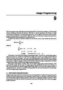
Note that G is bipartite with bipartition (X ∪Y ∪{vt : t ∈ F }, Z ∪{ut : t ∈ F }). Now we define b ∈ ZV such that but = 2 for each t ∈ F and bw = 1 for all other vertices w of G. Finally, we define a matrix A = (ave ) ∈ ZV ×E such that ave = 0 whenever v is not incident with e, ave = 2 whenever v = ut and e = (ut , vt ) for some t ∈ F , and ave = 1 otherwise; see Figure 1. It is straightforward to verify that (X, Y, Z, F ) is a yes-instance of the 3D Matching problem if and only if there exists x ∈ ZE satisfying (Ax = b, x ≥ 0). Now A and b are not (0, ±1)-valued, but if, for each t ∈ F , we subtract the vt -row from the ut -row, then the entries in the resulting system A′ x = b′ are in {0, ±1}.

INTEGER PROGRAMMING AND BRANCH-WIDTH

111111111 000000000 X 000000000 111111111 x 000000000 111111111 000000000 111111111 1 1 000000000 111111111 000000000 111111111 000000000 111111111 000000000 111111111

1 2

1 ut

2

9

11111111Y 00000000 00000000 11111111 y 00000000 11111111 1 00000000 11111111 1 00000000 11111111 00000000 11111111 00000000 11111111 00000000 11111111

1 1 vt 1

11111111 00000000 1 00000000 11111111 z 1 00000000 11111111 00000000 11111111 00000000 11111111 00000000 11111111 00000000 11111111 00000000Z 11111111 Figure 1. The reduction It remains to verify that M(A) is graphic. It is straightforward to verify that A is equivalent, up to row and column scaling, to a {0, 1}matrix A′′ . Since G is bipartite, we can scale some of the rows of A′′ by −1 to obtain a matrix B with a 1 and a −1 in each column. Now M(B) = M(A) is the cycle-matroid of G and, hence, M(A) is graphic.  6. Bounded variables In this section we consider integer programs with bounds on the variables. Integer programming with variable bounds (BIP) Instance: Positive integers m and n, a matrix A ∈ Zm×n , a vector b ∈ Zm , and vectors c, d ∈ Zn . Problem: Find x ∈ Zn maximizing ct x subject to (Ax = b, 0 ≤ x ≤ d). We can rewrite the problem as: Find y ∈ Z2n maximizing cˆt y subject ˆ = ˆb, y ≥ 0), where to (Ay       A 0 b c ˆ ˆ A= ,b= , and cˆ = . I I d 0 Note that, for i ∈ {1, . . . , n}, the elements i and i + n are in series ˆ and, hence, M(A) ˆ is obtained from M(A) by a sequence of in M(A),

10

CUNNINGHAM AND GEELEN

series-coextensions. Then it is easy to see that, if the branch-width of ˆ is at most max(k, 2). M(A) is k, then the branch-width of M(A) ˆ Therefore, Now note that the all-ones vector is in the row-space of A. ˆ by taking appropriate combinations of the equations Ay = ˆb, we can ˜ = ˜b where A˜ is non-negative. Therefore, make an equivalent system Ay we obtain the following corollary to Theorem 1.2. Corollary 6.1. There is a pseudopolynomial-time algorithm for solving (BIP) on instances where the branch-width of M(A) is constant. Acknowledgement We thank Bert Gerards and Geoff Whittle for helpful discussions regarding the formulation of Problem 1.5 and the proof of Theorem 1.4. References [1] B. Courcelle, “Graph rewriting: An algebraic and logical approach”, in: Handbook of Theoretical Computer Science, vol. B, J. van Leeuwnen, ed., North Holland (1990), Chapter 5. [2] W.H. Cunningham, Improved bounds for matroid partition and intersection algorithms, SIAM J. Comput. 15 (1986), 948-957. [3] M.R. Garey and D.S. Johnson, Computers and Intractability. A guide to the theory of NP-completeness, A series of books in the mathematical sciences, W.H. Freeman and Co., San Francisco, California, 1979. [4] P. Hlinˇen´y, Branch-width, parse trees and monadic second-order logic for matroids, manuscript, 2002. [5] G.S. Lueker, Two NP-complete problems in non-negative integer programming, Report No. 178, Department of Computer Science, Princeton University, Princeton, N.J., (1975). [6] S. Oum and P. D. Seymour, Approximating clique-width and branch-width, J. Combin. Theory, Ser. B 96 (2006), 514-528. [7] S. Oum and P. D. Seymour, Testing branch-width, to appear in J. Combin. Theory, Ser. B. [8] J. G. Oxley, Matroid Theory, Oxford University Press, New York, 1992. [9] C.H. Papadimitriou, On the complexity of integer programming, J. Assoc. Comput. Mach. 28 (1981), 765-768. [10] N. Robertson and P. D. Seymour, Graph Minors. X. Obstructions to tree-decomposition, J. Combin. Theory, Ser. B 52 (1991), 153– 190. [11] N. Robertson and P. D. Seymour, Graph Minors. XVI. Excluding a non-planar graph, J. Combin. Theory, Ser. B 89 (2003), 43-76.

INTEGER PROGRAMMING AND BRANCH-WIDTH

11

[12] P. D. Seymour, Decomposition of regular matroids, J. Combin. Theory, Ser. B 28 (1980), 305–359. [13] W. T. Tutte, A homotopy theorem for matroids, I, II, Trans. Amer. Math. Soc. 88 (1958), 144–174. Department of Combinatorics and Optimization, University of Waterloo, Waterloo, Canada N2L 3G1