On-line Anomaly Detection of Deployed Software: A ... - CiteSeerX

On-line Anomaly Detection of Deployed Software: A Statistical Machine Learning Approach George K. Baah, Alexander Gray, and Mary Jean Harrold College of Computing Georgia Institute of Technology Atlanta, GA 30332, USA

{baah|agray|harrold}@cc.gatech.edu

ABSTRACT This paper presents a new machine-learning technique that performs anomaly detection as software is executing in the field. The technique uses a fully observable Markov model where each state in the model emits a number of distinct observations according to a probability distribution, and estimates the model parameters using the Baum-Welch algorithm. The trained model is then deployed with the software to perform anomaly detection. By performing the anomaly detection as the software is executing, faults associated with anomalies can be located and fixed before they cause critical failures in the system, and developers time to debug deployed software can be reduced. This paper also presents a prototype implementation of our technique, along with a case study that shows, for the subjects we studied, the effectiveness of the technique. Categories and Subject Descriptors: D.2.5 [Software Engineering]: Testing and Debugging—Diagnostics, Monitors General Terms: Algorithms, Experimentation Keywords: Anomaly detection, Markov models, machine learning, fault localization, anomaly diagnosis

1. INTRODUCTION One of the challenging problems in software engineering is debugging of deployed software systems. Such systems are difficult to debug because they lack the mechanisms to inform developers or users when the software is behaving anomalously, and if so, which part of the software is responsible for the anomaly. For these systems, the only indication of anomalous behavior is a software crash or an observation by the user (typically by manual inspection) that an incorrect output has occurred. The lack of such mechanisms lets non-crashing faults, which can later cause significant failures, go undetected. The typical way to assist in locating faults in deployed

Permission to make digital or hard copies of all or part of this work for personal or classroom use is granted without fee provided that copies are not made or distributed for profit or commercial advantage and that copies bear this notice and the full citation on the first page. To copy otherwise, to republish, to post on servers or to redistribute to lists, requires prior specific permission and/or a fee. SOQUA’06, November 6, 2006, Portland, OR, USA. Copyright 2006 ACM 1-59593-584-3/06/0011 ...$5.00.

software is to log information as the system executes, and later, when a failure occurs, a developer, with the aid of automated tools, examines the logged information to find the cause of the failure. Because in practice it is not possible to store all execution information that the software produces, only partial execution information is stored. Thus, there is no guarantee that the information required to determine the cause of the failure will be present in the data gathered. Even if it were possible to gather all execution information, inordinate developer time and effort may be required to analyze the data, resulting in significant productivity loss. Furthermore, approaches that require complete executions or crashes miss opportunities to detect anomalous (possibly faulty) behavior early in the execution, and fix them before critical failures actually do occur. Therefore, to effectively debug deployed software, techniques must be able to detect anomalies, which might be correlated with faults, as the software is executing (i.e., perform on-line anomaly detection). Significant research has been performed in classifying software executions, without actually knowing the outcome, using machine-learning techniques. The techniques first build models, using approaches such as Markov modeling [1], construction of random forests [7], and clustering [4, 5, 9, 12], from execution information gathered on a training set of executions (i.e., test cases). The techniques then use the models to classify new executions into categories such as “passing,” “failing,” or “anomalous.” These existing classification techniques have three major limitations that make them unsuitable for use with deployed software. The first limitation is that the techniques cannot perform the classification of an execution until the complete execution has occurred because they require gathering of the execution information about the entire execution before they can perform their analysis. In practice, it may be difficult to gather and store the execution information required for the classification because large and long-running systems can produce inordinate amounts of execution information. Furthermore, because the techniques require complete execution information before being able to perform the classification, they cannot detect anomalous or failing behavior as the software is executing, and thus, may miss the opportunity to detect anomalies or symptoms of a given failure before the failure actually occurs. The second limitation is that, even if they were able to gather the execution information and classify the execution as “anomalous” or “failing,” the techniques have no means of detecting where the anomaly or failure

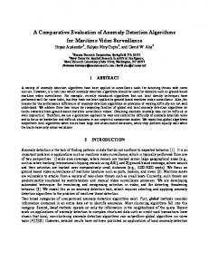
(a) Training Phase

(b) Deployment Phase

Figure 1: Our two-phase approach for on-line anomaly detection: the training phase (a) and the deployment phase (b). manifested itself in the software. The inability of the techniques to determine where such manifestations occur limits their usefulness for debugging deployed software. The third limitation is that, to produce effective models, the existing techniques require the availability of both passing and failing executions. In practice, it may be difficult to obtain failing executions on software that is ready for deployment because software companies rarely deploy software with known critical bugs. Capture-replay techniques (e.g., [10, 14]) have been proposed as an alternative to debugging deployed software systems. The techniques capture software executions that are then replayed at a later time when a failure occurs. The goal is to reproduce the conditions under which the failure occurred. Because the techniques cannot know where a fault is located in the system, to reproduce the conditions under which a failure occurred, they require storing large amounts of execution information, which make them unsuitable for use on deployed systems. There has been limited work in on-line anomaly detection of software. Hangal and Lam [6] present a technique that aims to address debugging of deployed software. The technique computes dynamic invariants as the software executes and uses the invariants to perform on-line anomaly detection and fault localization. Dynamic invariant detection reportedly adds significant overhead to an executing system, and thus, it might not be sufficiently efficient for use on deployed systems. Furthermore, the empirical studies on this technique are insufficient to determine the effectiveness in detecting anomalies (other than invariant violations) as the software executes. To address the limitations of existing techniques for use in on-line anomaly detection of deployed software, we have developed, and present in this paper, a novel machine-learning approach that detects anomalies as the software executes and assists in locating the part of the software that caused the anomaly. Our technique uses a fully observable Markov model [13] where each state in the model emits a number of distinct observations according to a probability distribution. Although each state has a number of observations, the observations are unique to each state: each observation belongs to only one state. The model parameters are estimated by using the Baum-Welch algorithm [13], which is a standard machine-learning algorithm for estimating parameters of the hidden Markov model [13]. The trained model can be deployed with the software to perform on-line anomaly

detection as the software executes. The main benefit of our technique is that it performs the anomaly detection and simultaneously locates where the anomaly manifests itself in the software as the software is executing in the field. Thus, anomalous behavior can be detected early in the execution, and faults can be located (i.e., if anomalous behavior is actually faulty behavior) possibly before they cause critical failures in the system. Furthermore, by detecting anomalies that are real failures during execution of the software, developers time to debug the system can be significantly reduced. Another important benefit of our approach is that it can create effective models using only passing test cases instead of using both passing and failing test cases, which is required, for building effective models, by existing techniques. In practice, there are many passing test cases for a system. However, when the system is ready for deployment, many of the faults, especially critical ones, have been fixed, and thus, there may be few failing test cases that can be used for the modeling. Building models with few failing test cases is most likely to result in poor models because there is no guarantee that the number of failing test cases covers a large portion of the state space. Building models with failing test cases is also not helpful unless the behaviors of the failing test cases can be generalized to other failures. In general, different failures occur in a variety of ways, thus, inducing different behaviors. The main contributions of this paper are: • A description of a novel technique that uses a fully observable Markov model to automatically perform anomaly detection and identify, as the software is executing, the part of the software where the anomaly manifested itself. • An overview of a prototype implementation of our technique that consists of two main components: instrumentation and learning • The results of case studies that show, for the subject program considered, that the technique was effective in detecting anomalies as the program executes. For the 33 seeded faults across the four versions of the subject program considered, our approach was able to detect all failing executions in 24 of them as anomalous. Furthermore, our approach was able to detect some of the failing executions in seven others as anomalous.

Figure 2: A sample program (left of table) with test inputs and predicate states produced by the program with those inputs (right of table).

2. APPROACH Our approach for performing on-line anomaly detection consists of two main phases: training and deployment. Figure 1 gives an overview of our technique using a data-flow diagram,1 where the training phase is shown in (a) and the deployment phase is shown in (b). This section discusses the details of each phase in turn.

2.1 Training Phase The training phase consists of three main steps: instrumentation, execution, and learning. For a program P that is to be monitored, the instrumentation step inserts probes into P to produce the instrumented program Pˆ . During the execution step, Pˆ is executed on the test suite T . The probes in Pˆ gather traces of predicate information2 that are then translated into states we call predicate states (we define and discuss the predicate states and their representation in detail in the next section). The predicate state traces are then input to the learning step that produces a model M . The important steps of the training phase are the execution and the learning. The rest of this section discusses the execution and the learning steps.

2.1.1

Execution Step

The significant activity that occurs during the execution step is translating the predicate information into a predicatestate representation. Our technique uses a predicate-state representation to capture partial semantics of the program. Our intuition is that the representation can capture behaviors among predicates and that information can be used to 1 In the data-flow diagram, the rounded rectangles represent processes, boxes represent external entities, arrows indicate the direction of flow of data, and labels on the arrows indicate the type of information. 2 The predicate information contains the values of the operands of the predicate, the predicate operator, the class name, the method name, and the line number where the predicate occurs.

recognize anomalous behaviors. Our intuition about the effectiveness of the predicate state representation is motivated by Pasareanu and collegues [11] through their work on the use of an under-approximated form of predicate abstraction. Their technique stores the abstract states corresponding to the concrete states of the program executions. Our technique takes the same approach: instead of storing the concrete states of the program executions, our technique stores the predicate states corresponding to their respective concrete states. To construct the states, our approach first analyzes the program to extract its predicates. The technique then groups together the predicates according to their methods; we group the predicates according to their methods because the effects of most predicates tend to be local to where they are defined. The technique later analyzes the methods and constructs a state representation for each method using the predicates in the method. We call an instance of a predicate state representation a predicate state. A predicate state is a 4-tuple defined by (cn,mn,ln,vp): cn, mn, and ln, are the class name,3 method name, and line number associated with the state, respectively; vp represents the interactions among the predicate values in mn at ln. Each predicate can assume three values: T , when the predicate evaluates to “true;” F , when the predicate evaluates to “false;” and ∗, when the predicate has not been executed. A predicate is active if it has been executed at least once regardless of its outcome (i.e., T or F ). Because errors tend to occur at boundaries of conditions we let vp capture boundary information. Thus, if a predicate symbol is either ≤ or ≥, we split the predicate into two predicates. For example, our technique translates (x ≤ y) to (x < y) and (x == y). Also, if a predicate symbol is either > or y), 14(x > z). However, because the predicate symbols are all P (Otsi |M ) > > > > > (2) T hreshold(sj , si ) = min : sj ; (sj ,si ) P (Ot−1 |M ) where P (Otsi |M ) is the joint probability of the predicate states with the last predicate state at time t being emitted sj from state si . P (Ot−1 |M ) represents the joint probability of the sequence of predicate states up to time t − 1 with the predicate state at t − 1 being emitted from state sj . M represents the model parameters. Any execution that traverses the two states and violates the threshold between the two states is flagged as anomalous. The joint probability for each sequence of predicate states is computed using the forward algorithm [13]. The forward algorithm, is a standard algorithm used to compute the probability of a sequence of observations in the hidden Markov model literature [13]. After the thresholds have been determined, the model is deployed with the software. Note that the threshold between si and sj is not the same as the probability of transitioning between the two states. The probability of transitioning from si to sj is obtained directly from the model’s statetransition-probability distribution. Also the probability of transitioning from si to sj is used directly by the forward algorithm to compute the joint probability of the predicate state sequences. In our implementation the probabilities

are converted into logarithmic form because the probabilities tend to be very small.

2.2

Deployment Phase

During the deployment phase, as illustrated in Figure 1, the model M is deployed with the instrumented program Pˆ . The execution information produced by Pˆ as it executes in the field is analyzed by M to simultaneously detect anomalies and identify the location in the software code where the anomalies manifest themselves. The results of the analysis of M , which are the locations in the software where the anomalies occurred, are presented to the user or developer. The developer can then use various off-line faultlocalization techniques (e.g., [2, 8] to investigate the cause of the anomaly.

Anomaly Detection After the model has been deployed with the instrumented software, for each time step t in the execution of the software the joint probability ratio between the current and previous predicate state sequences is computed. The joint probability ratio becomes the current value between the states of the predicate states at the current and previous time. Let Dt (sj , si ) represent the current ratio between sj and si at time t during execution of the software then, 8 9 > P (Otsi |M ) > > > > > Dt (sj , si ) = : (3) sj ; P (Ot−1 |M ) where sj and si are the states at the previous and current time respectively. P (Otsi |M ) is the joint probability of the current predicate state sequence with the last predicate state sj at the current time t being emitted from si . P (Ot−1 |M ) represents the joint probability of the previous predicate state sequence up to previous time t − 1 with the predicate state at t − 1 being emitted from sj . M represents the model parameters. At any given time in the execution of the software if Dt (sj , si ) < T hreshold(sj , si ), the execution is flagged as anomalous. Note that the joint probability is computed on-line using the forward algorithm [13]. Also the probability of the previous predicate state sequence has already been computed thus, making it a constant in Equation 3 at the current time t. If the program, Mid, is deployed with its current model and it receives Input 2, the model traverses the path (s4 → s5 → s7 ), indicated by the thick black arrows in Figure 3. As the model traverses the path, it computes the joint probability of the predicate states emitted as the model transition goes from s4 , to s5 and finally to s7 , using the forward algorithm. When Input 3 is applied to the program, transition goes from s4 to s5 to A because the last state “7,[T,F,F,F,T,F,*,*,*,*]” had not been encountered during the training of the model. The transition to A automatically causes the execution to be flagged as anomalous.

3.

CASE STUDIES

To evaluate the effectiveness of our approach, we implemented a research prototype and conducted two case studies. The prototype consists of two parts: instrumentation and learning. The instrumentation part consists of a Java program instrumenter based on the Soot framework [15]. The machine-learning part is implemented in the Ocaml language, and consists of two modules: learning and anomaly

Figure 4: Anomaly detection results for NanoXML. detection. The learning module is used during the building of the Markov model and the anomaly detection module is used when the model is deployed with the program. All implementation are unoptimized at this time. As a subject for our studies, we use NanoXML, which is an XML parser for Java. NanoXML has five versions, each of which contains between 16 and 23 classes and between 4K and 7K lines of code. Each version comes with seeded faults, which can be activated individually. For our study we omitted version 4 because it has no seeded faults. In total, there are 33 seeded faults across the four versions we considered. Each version has between 214 and 216 test cases, and there is a fault matrix associated with each version that indicates which test cases pass and which test cases fail.

3.1 Study 1 The goal of this study was to determine the on-line anomaly detection capability of our approach. To do this, for each version of NanoXML, we first activated each of the faults individually. When a fault was activated for a given version, we instrumented the version and executed the passing test cases on the version to collect traces of predicate states. The predicate state traces were input to the learning module to produce the model for the version. After the model was built, the failing test cases from the version’s test suite were then executed on the instrumented version and the predicate state traces generated were input to the anomaly detection module, which consists primarily of the model, to perform on-line anomaly detection. The graph in Figure 4 shows the results of this study. The horizontal axis represents the version number (i.e., v#) of NanoXML, the fault number (i.e., b#), and the number of failed test cases for each fault number. The vertical axis shows the percentage of failing test cases our technique was able to detect as anomalous before execution of the pro-

gram ended. For example, from the graph, version 1 with fault number 2 (i.e., v1b2) has 44 failing test cases. Our technique detects 11 of the failing test cases as anomalous before execution of the failing test cases on v1b2 completes. Therefore, the height of the bar shows 25% (11/44), which is the percentage of failed test cases our technique detected as anomalous before execution of the test cases completed. Overall, our technique was able to detect anomalies in all versions (with most of them being 100%), with their activated faults, except v1b2, v1b3, v1b4, and v3b5 which have detection rates below 50%. The detection rate of our technique was below 50% for v1b2, v1b3, v1b4, and v3b5 because our technique best detects faults that are domain errors [16]. The faults in v1b2, v1b3, v1b4, and v3b5, in certain executions, behave like computation errors [16] and sometimes like domain errors. Thus, our technique could not fully detect anomalies induced by these errors. When the error is a computation error the technique is most likely to have a 0% detection rate. The first-order Markov assumption inherent in our model means the probability of the current state is independent of all past states except the previous state. This assumption directly affects the threshold values because the thresholds will not reflect the long-range dependencies among the states. These long-range dependencies may be needed to improve the recognition of anomalous executions (which may be be failing). Another observation is that our model is not capturing direct dependencies among predicate states. Instead it only captures dependencies among adjacent states. The lack of direct dependencies also affects the threshold values.

3.2

Study 2

The goal of this study was to determine whether there were any advantages to using line-number clustering over

method clustering in terms of anomaly-detection capabilities. We used the same subject program and setup as in Study 1. The result shown in Figure 4 was obtained using linenumber clustering for the subject program. Method clustering is at a higher abstraction than line-number clustering and thus, we expected the results of line-number clustering to be better than method clustering. Our results showed, however, that there was no advantage in using line-number clustering over method clustering in terms of anomaly detection capabilities for the subject program considered because the anomaly-detection results were the same for both clustering techniques. The anomaly-detection rates were the same because the errors in the versions of the subject program were domain errors [16] that our predicate state representation was able to capture. The capturing of the behavior of the domain errors resulted in new predicate states that the model had not encountered before, hence causing the executions to be flagged as anomalous by the models for both clustering techniques. Our results also show that, whereas it took four hours to build the model using line-number clustering, it took only 22.1 minutes to build the model using method clustering. This difference in model-building time occurs because the line-number clustering had more states (on average, greater than 175) than method clustering (on average, 59 states). For other subject programs where no new predicate states are encountered, we expect the line-number clustering to be better than the method clustering because it is at a finer level of granularity than method clustering.

4. RELATED WORK Our work is related to previous research in software execution classification. Section 1 (Introduction) gave an overview of some of these techniques. This section provides a more detailed discussion of the techniques, and compares our work to them. There are a number of techniques for anomaly detection and classification of software executions (e.g., [1, 5, 7, 12]). These techniques use both passing and failing executions (test cases) for building their models. There are no empirical studies that demonstrate the effectiveness of the techniques when only passing executions are used. However, for deployed software, test suites for use in building classifiers may contain only passing test cases. Unlike these approaches, our technique is effective when only passing executions are available, although failing executions can be incorporated into our technique. We next present the mostclosely related techniques, and discuss additional ways that ours differs from theirs. Bowring and colleagues [1] use Markov models, constructed from profiles of program entities (e.g., branches and method calls), and build classifiers for predicting execution outcomes. Their technique requires that the software execute to completion before classification can be performed. Because debugging deployed software requires that classification be performed as the software executes, their approach is unsuitable. In contrast, our technique performs the classification as the software executes, and thus, can be used for detecting anomalies and locations where the anomalies manifest. Haran and colleagues [7] also present a technique based on machine-learning to build classifiers for software executions but theirs uses random forests instead of Markov mod-

els. Their model is also built using passing and failing test cases. To handle the significant amount of execution information produced by the software, their technique lightly instruments the software before it is deployed. Like Bowring and colleagues, their technique requires the software execution to complete before they can classify the execution. Large and long running software systems can still produce an inordinate amount of execution information even if the software is lightly instrumented. Thus, collection of all execution information from a field execution before classification may prohibit classification of large or long-running programs. Our technique avoids this cost because it performs the classification of the execution as the software executes. Our technique can also provide the location in the software code where the anomaly manifested itself. Podgurski and colleagues [5, 12] present techniques that use automated clustering, logistic regression, and software visualization to facilitate the debugging process by grouping together failing executions that have similar causes. Like the previously discussed techniques [1, 7], they require that the execution of the software completes before their technique can be applied. They also require that the executions be labeled before applying their technique. Thus, their technique is not suitable for deployed software. Our technique differs from theirs in that it performs anomaly detection and locates the location of the anomaly in the software code as the software executes, without requiring complete or externallylabeled executions. Hangal and Lam [6] present a technique that is close in spirit to our technique. Their technique is directed toward the debugging of deployed software. The technique computes dynamic invariants as the software executes, and the technique uses invariants to perform on-line anomaly detection and fault localization. Dynamic invariant detection reportedly adds significant overhead to an executing system, and thus, it might not be sufficiently efficient for use on deployed systems. Furthermore, the empirical studies on this technique are insufficient to determine how effective it is in detecting anomalies other than invariant violations. Our technique differs from their technique in that we build machine learning models of software execution. Our technique does not compute invariant information as the software executes but rather gathers predicate information. Our technique therefore has the potential to scale to large software systems and also to be efficient.

5.

CONCLUSION

In this paper, we have presented a new machine learning technique for on-line anomaly detection of deployed software. We implemented the technique and performed two case studies on a mid-sized Java program. Our empirical results show that our approach is promising and that, for our subject program, our technique is effective in detecting anomalies in the failing executions of the program. We have also shown that our technique can be effective when trained only on passing executions of the program. Also our studies show that, for the subject program considered, the different clustering techniques had no effect on the anomaly detection rate. However, we performed our studies on only one mid-sized subject program with many fault-seeded versions. The results do not show whether our technique will scale to larger programs. We will continue to perform studies on additional

subjects with different sizes to determine the technique’s effectiveness and to guide our future research. Our empirical studies also showed that our approach works well for particular types of bugs—those that are domain errors [16] or those where a computation error [16] later affects a path condition. In these cases, our anomaly detection flagged the execution and our technique was able to help locate the part of software code where the anomaly manifested itself. We are currently working on enhancing the information we record and the modeling technique to account for errors caused by computations that do not influence the path condition. The first-order Markov assumption inherent in our model, which was explained earlier, has an effect on the threshold values. The thresholds fail to capture the direct dependencies among predicates states, and also long-range dependencies among the states in the model. To improve the thresholds, we are exploring additional machine learning models that do not suffer from the first-order Markov model assumption. Also better test suites imply better thresholds and therefore, we intend to improve the test suites of subject programs considered. We also plan to investigate types of test-suite development and coverage techniques that would lead to good models. In future work, we will extend this technique by incorporating fault-localization capabilities into the technique. Incorporating fault-localization capabilities into our technique is possible because when an anomaly manifests itself, the technique pinpoints exactly where the anomaly occurred in the software. The use of fault-localization techniques such as Cause Transitions [2] and Tarantula [8] can make it possible to localize errors if the anomaly happens to be caused by a real fault. There are two efficiency issues our technique must overcome so that it can be useful in practice. The first efficiency issue concerns the time required to build the models especially in the presence of large test-suite sizes. To address this issue, we will explore active-learning [3] for building our models. For future work, we will also be exploring the use or development of on-line machine learning algorithms. We are currently exploring other clustering techniques that can effectively deal with the predicate-states explosion problem. The second efficiency issue concerns the cost of instrumenting the software to gather more information without incurring significant overhead, and how quickly the model can track the execution of the software. Ideally, we want to have the on-line anomaly detection of the software execution to be real-time (i.e., the model detection speed is in step with the software execution). To address this second issue we are investigating the use of hardware techniques to make our implementation more efficient at gathering execution information, and also to increase the speed of the on-line anomaly detection of the model.

6. REFERENCES [1] J. F. Bowring, J. M. Rehg, and M. J. Harrold. Active learning for automatic classification of software behavior. In Proceedings of the international symposium on software testing and analysis, July 2004. [2] H. Cleve and A. Zeller. Locating causes of program failures. In Proceedings of the International Symposium on the Foundations of Software Engineering, pages pages 342–351, May 2005.

[3] D. A. Cohn, L. Atlas, and R. E. Ladner. Improving generalization with active learning. In Machine Learning, volume 15, pages 201–221, 1994. [4] W. Dickinson, D. Leon, and A. Podgurski. Pursuing failure: the distribution of program failures in a profile space. In Proceedings of the 8th European Software Engineering Conference held jointly with 9th ACM SIGSOFT International Symposium on Foundations of Software Engineering, September 2001. [5] P. Francis, D. Leon, M. Minch, and A. Podgurski. Tree-based methods for classifying software failures. In Proceedings of the 15th International Symposium on Software Reliability Engineering, November 2004. [6] S. Hangal and M. Lam. Tracking down software bugs using automatic anomaly detection. In Proceedings of the 24th international conference on software engineering, pages 291–301, May 2002. [7] M. Haran, A. Karr, A. Orso, A. Porter, and A. Sanil. Applying classification techniques to remotely-collected program execution data. In Proceedings of the European Software Engineering Conference and ACM SIGSOFT Symposium on the Foundations of Software Engineering (ESEC/FSE 2005), pages 146–155, September 2005. [8] J. Jones and M. J. Harrold. Empirical evaluation of the tarantula automatic fault-localization technique. In Proceedings of the 20th IEEE/ACM International Conference on Automated Software Engineering, November 2005. [9] D. Leon, A. Podgurski, and L. J. White. Multivariate visualization in observation-based testing. In Proceeding of the 22nd International Conference on Software Engineering, May 2000. [10] A. Orso and B. Kennedy. Selective capture and replay of program executions. In Proceedings of the Third International ICSE Workshop on Dynamic Analysis (WODA 2005), pages 29–35, May 2005. [11] C. Pasareanu, R. Pelanek, and W. Visser. Concrete model checking with abstract matching and refinement. In Proceedings of 17th international conference on computer-aided verification, July 2005. [12] A. Podgurski, D. Leon, P. Francis, W. Masri, M. M. Sun, and B. Wang. Automated support for classifying software failure reports. In Proceedings of the 25th International Conference on Software Engineering, May 2003. [13] L. R. Rabiner. A tutorial on hidden markov models and selected applications in speech recognition. In Proceedings of IEEE, volume 77, pages 257–286, February 1989. [14] J. Steven, P. Chandra, B. Fleck, and A. Podgurski. jrapture: A capture/replay tool for observation-based testing. In Proceedings of International Symposium on Software Testing and Analysis, 2000. [15] R. Vallee-Rai, P. Co, E. Gagnon, L. Hendren, P. Lam, and V. Sundaresan. Soot - a java bytecode optimization framework. In CASCON ’99: Proceedings of the 1999 conference of the Centre for Advanced Studies on Collaborative research, page 13, 1999. [16] S. J. Zeil. Perturbation techniques for detecting domain errors. In IEEE Transactions on Software Engineering, volume 15, pages 737–746, June 1989.