On-line approximate string matching in natural

Fundamenta Informaticae 72(4): 453–466 IOS Press

On-line approximate string matching in natural language Kimmo Fredriksson∗ Department of Computer Science University of Joensuu PO Box 111, 80101 Joensuu, FINLAND [email protected]

Abstract. We consider approximate pattern matching in natural language text. We use the words of the text as the alphabet, instead of the characters as in traditional string matching approaches. Hence our pattern consists of a sequence of words. From the algorithmic point of view this has several advantages: (i) the number of words is much less than the number of characters, which in effect means shorter text (less possible matching positions); (ii) the pattern effectively becomes shorter, so bit-parallel techniques become more applicable; (iii) the alphabet size becomes much larger, so the probability that two symbols (in this case, words) match is reduced. We extend several known approximate string matching algorithms for this scenario, allowing k insertions, deletions or substitutions of symbols (natural language words). We further extend the algorithms to allow k 0 errors inside the pattern symbols (words) as well. The two error thresholds k and k 0 can be applied simultaneously and independently. Hence we have in effect two alphabets, and perform approximate matching in both levels. From the application point of view the advantage is that the method is flexible, allowing simple solutions to problems that are hard to solve with traditional approaches. Finally, we extend the algorithms to handle multiple patterns at the same time. Depending on the search parameters, we obtain algorithms that run in linear or sublinear time and that perform the optimal number of word comparisons on average, We conclude with experimental results showing that the methods work well in practice.

Keywords: Approximate string matching; filtering; natural language processing; phrase matching; word alphabet. Address for correspondence: Kimmo Fredriksson, PO Box 111, 80101 Joensuu, FINLAND. Supported by the Academy of Finland, grant 202281.

∗

453

454

K. Fredriksson / On-line approximate string matching in natural language

1. Introduction String matching is to find the exact or approximate occurrences of the given pattern P from the text T , where P and T are sequences of symbols drawn from some alphabet. Classical string matching algorithms are usually applied in character level, that is, the underlying alphabet is considered to be some small set of characters, such as ASCII or DNA alphabet. This is very natural way to apply the algorithms, but in some applications one can define ’higher order’ alphabets as well. In particular, natural language texts are sequences of words (and separators between the words), which can be seen as symbols of a huge alphabet, or vocabulary. We show that this view leads to efficient approximate string matching algorithms for natural language texts. Besides being fast, the method is also very flexible, allowing efficient solutions for many problem variations that are hard to solve with the traditional (see [15] for references) approaches. Given a pattern P of m words, and a text T of n words, and parameters k, k 0 , and r, we consider the following problems: • Find the occurrences of P from T , allowing at most k insertions, deletions or substitutions of words. • As above, but simultaneously allow at most k 0 insertions, deletions or substitutions of characters for each word in P . • As above, but search r patterns simultaneously. We also consider two special cases, giving more efficient algorithms for them: (i) k = 0, k 0 ≥ 0; (ii) m = 1 (i.e. the pattern is a single word, implies k = 0). All the algorithms can be extended in many ways with little additional cost, such as removing stop words, or even adding thesaurus such that a word in P can match also its synonym word in T . Our technique of moving to word alphabet is related to the string matching algorithm for word-based Huffman compressed texts [11], which relies on the availability of the whole text vocabulary in the Huffman tree. Depending on the algorithms, we either do not need the vocabulary, or build (possibly only a fraction of) it on-line with lazy evaluation as needed. The proposed algorithms run in linear or sublinear time on average, depending on the search parameters.

2. Problem definition P Formally, define the text string T1..n = W1 S1 W2 S2 ...Sn−1 Wn , where Wi ∈ Σ∗ , Si ∈ ∆∗ , and i |Wi |+ P i |Si | = N . Σ and ∆ are some finite alphabets, of size σ and δ respectively. That is, we have a (natural language) text that consist of n words, separated by n − 1 separators, whose combined total length is N characters. In our context Σ ∪ ∆ can be seen e.g. as the standard ASCII alphabet. We use Λ to denote our word alphabet, and λ = |Λ| is the size of the alphabet, i.e. the total number of distinct words in T and P . By Heaps’ law, λ = nβ , where β = 0.4...0.6 for English language [7]. Further, we have a pattern string P1..m , where Pi ∈ Σ∗ . That is, P is a sequence of words. If needed, P may contain also separators just as well, but this is usually not interesting. The total length of P is


455

P

i |Pi | = M characters. We use b to denote the average length of the words in T and P , that is, we assume that b = M/m = N/n. In practice b can be regarded as a small language dependent constant. Exact matching is then to find all the text word positions i where Wi−j+1 = Pm−j+1 , for j = 1..m. Edit distance ed(A, B) between strings A and B is defined as the minimum number of edit operations that are needed to convert string A into string B, where the allowed edit operations are substitution, insertion or deletion of one string symbol. If the symbols are words, we use the notation ed, and for single character symbols the notation ed0 . The edit distance ed(A, B) can be efficiently computed by dynamic programming. The algorithm fills a table D0..|A|,0..|B| , where each value Di,j corresponds to ed(A1..i , B1..j ), and eventually ed(A, B) = D|A|,|B| . When the values Di−1,j−1 , Di,j−1 and Di−1,j are known, the value Di,j can be computed by using the following well-known recurrence:

Di,0 = i. D0,j = ( j. Di,j =

D[i − 1, j − 1], if Ai = Bj . 1 + min(Di−1,j−1 , Di−1,j , Di,j−1 ), otherwise.

In word level approximate matching we report the word positions i where ed(P1..m , Wj..i ) ≤ k, for some j, where 0 ≤ k < m. Independently and simultaneously, we can allow character level approximate matching. Any two given words Wi and Pj are defined to match, if ed0 (Wi , Pj ) ≤ k 0 . In what follows, we consider two problem variations where (i) k ≥ 0 and k 0 = 0; and (ii) k ≥ 0 and k 0 ≥ 0. Exact matching is handled as a special case of (i). We also consider multiple pattern matching, where we search r patterns simultaneously, and the special case of m = 1, i.e. the patterns consist of single words.

3.

Algorithms

The edit distance computation can be easily modified to find approximate occurrences of P from T [16]. The only modification needed is to change the boundary condition D0,j = j into D0,j = 0. In this case Dm,j = min(ed(P1..m , Th..j ), h ≤ j). This gives immediately our first algorithm for word level approximate matching (k ≥ 0, k 0 = 0): report all j such that Dm,j ≤ k. The running time of this algorithm is O(N + nmb) which is equal to O(N m) or O(N + nM ), since we need O(N ) time to scan all the characters of the text, there are nm word pairs to compare, and each comparison takes O(b) time in the worst case. However, on average, the comparison between two random words takes only O(1) time, so the expected time is O(N + nm). The well-known “cut-off” heuristic [18] can be used to improve this. The heuristic uses the fact that on average we must evaluate only O(k) rows for each column of the matrix to see that the match cannot end at the current column. This directly gives us O(N + nk) expected time algorithm (assuming again that word comparison takes O(1) time on average).

3.1.

Augmented vocabulary

In order to improve the above results, we need an index structure for the distinct words in P (and/or in T ). We need to do efficiently the following operations:

456


•

INSERT (I, A, x):

•

UPDATE (I, A, x):

•

QUERY (I, A):

insert the word A with satellite information x into the index structure I. update the satellite x corresponding to the already inserted word A.

return the satellite information associated with the word A.

These can be easily implemented using e.g. hashing or trie, requiring O(|A|) worst case time for all operations. The following algorithms will insert all the distinct words of P (and/or T ) into this data structure.

3.2.

Bit-parallel dynamic programming

One of the properties of the matrix D is that the adjacent (horizontal, vertical or diagonal) values can differ at most by ±1: ∆hi,j

= Di,j − Di,j−1 ∈ {−1, 0, +1}

∆vi,j

= Di,j − Di−1,j ∈ {−1, 0, +1}

∆di,j

= Di,j − Di−1,j−1 ∈ {0, 1}

It is clear that these vectors fully define the matrix D, and any value Di,j can be obtained e.g. as follows: i X Di,j = ∆vs,j . s=1

In [12, 8] it was shown how to compute the vectors ∆h, ∆v, ∆d bit-parallely, in time O(ndm/we), where w is the number of bits in a computer word. Each vector ∆h, ∆v, ∆d is now represented by the following bit-vectors: HPi,j

≡ ∆hi,j = +1

HNi,j

≡ ∆hi,j = −1

V Pi,j

≡ ∆vi,j = +1

V Ni,j

≡ ∆vi,j = −1

D0i,j

≡ ∆di,j = 0

The values of these vectors can be computed very efficiently using bit-wise logical operations, bit shifts and additions, w vector elements in O(1) time, leading to a O(ndm/we) time algorithm. Alg. 2 shows the logical equivalencies and details of updating the vectors, using C-like bit-wise operations. The comparisons (Pi = Tj ) are implemented parallely using preprocessed bit masks P Mi,j ≡ Pi = Tj . For correctness and more details, refer to [12, 8]. In principle, there is nothing that prevents us using this algorithm for word based matching. The only obstacle is the preprocessing of the vectors P M . The original method preprocesses a table that has one P M vector entry for each possible character in the alphabet: iff P M [c] has bit 1 in position i, then the character c matches the pattern at position i. This is hardly possible in our case, as the alphabet size is huge. We therefore build the P M vectors only for those words that actually appear in P at some position. We insert each word in P into our index structure, with its preprocessed P M vector. Alg. 1 shows the


457

pseudo code. In the search phase, we query this structure for each word Wi in T . If Wi appears in the index, then we use the stored P M vector, otherwise we know that the vector must have zeros in every position. Alg. 4 show the pseudo code. The running time of the algorithm is clearly O(N + n(dm/we + b)) = O(N + ndm/we). The O(N ) term comes from the fact that we have to parse the text to get the words Wi out of it (not shown in the pseudo code). Finally, it is easy to modify the algorithm to use the “cut-off” heuristic as well, so as to obtain a O(N + ndk/we) expected time algorithm. Theorem 3.1. For k > 0, k 0 = 0 Alg. 4 runs in O(N + ndk/we) average time.

3.3.

Errors inside words

The above algorithm allows k > 0, but requires that k 0 = 0. We now consider removing this restriction. Alg. 4 would still work, if Get-PM(I, Wi ) (line 4) returned P M vectors computed such that we allowed up to k 0 differences between the words. That is, the jth bit of P M is set, iff ed0 (Pj , Wi ) ≤ k 0 . We therefore replace the Alg. 3 with Alg. 5 (and omit Alg. 1). Instead of indexing the words in P , we index the words in T as we encounter them. For each word in T , the algorithm checks if it is already in the index, and if so, returns the corresponding P M vector. If not, it computes the P M vector for the pattern corresponding to the current text word, and inserts the word with its vector into the index. The distances ed0 (Pj , Wi ) can be computed bit-parallely in time O(bdb/we) with minor modifications to Myers’ approximate bit-parallel search algorithm. As we are only interested distances that are ≤ k 0 , this can be improved to O((k 0 + log b)db/we) expected time (in fact, slightly better bound can be obtained) with the bit-parallel technique of [10]. Alternatively, the O(k 0 2 ) time non-bit-parallel algorithm [18] can be used. We use the O(bdb/we) algorithm. The total running time of Alg. 4 then becomes O(N +ndm/we+λM db/we), where λ is the number of distinct words in T . Using the “cut-off” version again, the expected time becomes O(N + ndk/we + λM db/we)). If we make the very reasonable assumption that dk/we and db/we are O(1), then to keep the previous bound O(N + ndk/we) = O(N ), it is enough that λM < N , which according to Heaps’ law is the same as m < n1−β . In practice this holds almost always. We have obtained the following: Theorem 3.2. For k, k 0 > 0 Alg. 4 runs in O(N + ndk/we + nβ M db/we)) average time.

3.4.

Backward matching

We now consider the case k = 0, k 0 ≥ 0. Using the above technique of indexing the distinct text words, algorithms like BDM [4] and BNDM [14] for exact matching (k = 0) can be easily applied. We chose BNDM which is a bit-parallel version of BDM. BNDM is much simpler to implement and is in practice faster if w ≤ m (i.e. we have enough bits). The idea is to use an automaton that recognizes all the suffixes of the reverse pattern. The automaton is then used to scan a text window of m symbols backwards. If the whole window can be scanned without mismatches, then a pattern occurrence have been found. However, whether or not the pattern occurs in the current window, some of the occurrences may overlap that window. But in this case some of the suffixes of the reverse pattern must match, since the suffixes of the reverse pattern are the prefixes of the original pattern. Hence the algorithm remembers the longest suffix that matched the text window. The next text window to be checked is the one that has this suffix aligned in the left end of the window.

458


Alg. 1 BP-DP-P RE P ROC(P, m). Input: Pattern P , its length m. Output: Index I that stores the match vector P M for each word in P . 1 I=∅ // Initialize the index 2 for i ← 1 to m do // For all words in the pattern: 3 P M ← QUERY(I, Pi ) // Is Pi indexed yet? 4 if P M = null then // No, preprocess it: the i-th word matches... 5 P M ← 1 ¿ (i − 1) // ...so set the i-th bit of the match vector. 6 INSERT (I, Pi , P M ) // Store the match vector for Pi . 7 else // Pi occurs earlier in P as well... 8 P M ← P M | (1 ¿ (i − 1)) // ...so just update the match vector. 9 UPDATE (I, Pi , P M )

Alg. 2 U PDATE V ECTORS(P M, score). Input: P M , score Output: New value of score 1 D0 ← (((P M & V P ) + V P ) ∧ V P ) | P M | V N 2 HP ← V N | ∼(D0 | V P ) 3 HN ← V P & D0 4 V P ← (HN ¿ 1) | ∼(D0 | (HP ¿ 1)) 5 V N ← (HP ¿ 1) & D0 6 score ← score + ((HP À m) & 1) − ((HN À m) & 1)

Alg. 3 G ET PM(I, W ). Input: Index I, word W Output: If W occurs in P , then the corresponding match vector, otherwise a vector of zeros. 1 P M ← QUERY(I, W ) 2 if P M 6= null then return P M else return 0

Alg. 4 BP-DP-S EARCH(I, T, s, e). Input: Index I, text T , the starting and ending positions s and e for the search Output: j ∈ {s..e}, Dm,j | Dm,j ≤ k 1 V P ← ∼0, V N ← 0 2 score ← m // score = Dm,s 3 for j ← s to e do // For words s . . . e of T do: 4 P M ← G ET PM(I, Wi ) // Get the match vector for word W 5 U PDATE V ECTORS(P M, score) // Update ∆-vectors, score = Dm,j 6 if score ≤ k then print(j, score)


459

Alg. 5 G ET PM(I, W ). Input: Index I, word W Output: If W occurs in P with at most k 0 errors, then the corresponding match vector, otherwise 0 1 P M ← QUERY(I, W ) // W already indexed? 2 if P M 6= null then return P M // Yes, return the match vector 3 PM ← 0 // W is a new word, initialize the match vector... 4 for i ← 1 to m do // ...compare all Pi against W : 5 if ed0 (Pi , W ) ≤ k 0 then // Do they match with at most k 0 errors? 6 P M ← P M | (1 ¿ (i − 1)) // Yes, update the match vector 7 INSERT (I, W, P M ) // Store the new word with the corresponding match vector. 8 return P M

BNDM has optimal [19] O(n logσ m/m) expected running time, assuming that m ≤ w. On average only O(logσ m) symbols are inspected in each window, and the average shift is O(m) symbols. See [14, 4] for more details. Alg. 6 gives the pseudo code. In our case this would mean O(n logλ m/m) expected number of word comparisons. However, note that the analysis assumes that each of the symbols appear with 1/λ probability, which is not true for real texts. By Zipf’s law [20] the ith most frequent word will appear 1/iθ times the frequency of the most frequent word, where θ is a small constant, ranging between 1.5...2 for English texts. Although this models the text itself very well, it is not true for the pattern. The reason is that the pattern is not likely to contain stop words like ’the’ or ’to’ and so on, which are the most common words in English language. In fact, real implementation of the search algorithm should just skip the stop words, not trying to match them against the pattern1 . One could further argue that the search pattern should typically contain words that are rare in the text. We therefore simply assume that the probability that two words match is p, and the algorithm therefore makes O(n log1/p m/m) word comparisons. The only complication with this approach is how to implement the shift. BNDM gives us the number s of words the window can be shifted. However, the text is a sequence of characters, and the word boundaries are not known, so the shift value cannot be directly used. A simple solution is to just scan the text from the current position, character by character, until s words are skipped. This means that the algorithm takes at least O(N + n log1/p m/m) time, and hence is not better than the basic dynamic programming approach (for m ≤ w). In practice BNDM is much faster, since it makes fewer word comparisons and needs to compute less P M vectors (Alg. 5), and the constant factor in the brute-force computing of the shifts is very small. An alternative way is to compute a tight lower bound for the number of characters to shift, given that we must shift s words. The following Lemma gives the needed bound: Lemma 3.1. To shift by s words, it is safe to shift by at least c =

m X i=m−s

(|Pi | + 1 − k 0 ) = s(1 − k 0 ) +

m X

|Pi | = O(M )

i=m−s

characters. 1

This is not always clear, consider the counter example: “to be or not to be”. This famous quote consists only of stop words...

460


Proof: Shifting by s words means that the algorithm has found a prefix of the pattern that matches with m − s words length suffix of the search window. For a pattern word to match a text word, its length must be at least |Pi | − k 0 characters, as otherwise the edit distance between the words must exceed k 0 . Moreover, each word is separated with a space, whose length is at least 1. u t After skipping c characters, we scan the text (character by character) to the next word boundary in O(b) time. What is remarkable here is that although c is a lower bound for the number of characters to shift, it may yield larger shift than the brute-force method, i.e. the number of words skipped with c characters can be larger than s, if the text words are short compared to pattern words. The shift can be implemented with a look-up table of size O(m). Analysis. By using Alg. 5 to compute the P M vectors for BNDM, we have an algorithm that allows k 0 ≥ 0 (but k = 0), and requires only O(n log1/p m/m) word comparisons on average, where p is the probability that two randomly picked words match with at most k 0 errors. By [1] the probability that two (fixed) randomly generated words of length b match with k 0 errors is O(γ b ), where 0 < γ < 1 given that √ k 0 /b < 1 − e/ σ. The fact that BNDM inspects only O(n log1/p m/m) words of the text on average means that the index construction of Alg. 5 takes only O((n log1/p m/m)β M db/we) time on average. The algorithm needs O(b) time to scan and compare each word. The shifting costs O(b) time per text window, for a total of O(nb/m) average time. The average running time of the algorithm therefore becomes O(nb/m + nb log1/p m/m) = O(N log1/p m/m), without the index construction. For k 0 > 0 the indexing of the text words takes O((n log1/p m/m)β M db/we) average time, negligible compared to the other costs. In the worst case this becomes O(λM db/we), where λ is the number of distinct words in the text. Note that db/we is √ O(1) for any real life text. We have obtained the following for k 0 < b(1 − e/ σ): Theorem 3.3. Alg. 6 runs in O(N log1/p m/m + (n log1/p m/m)β M db/we) average time. Finally, note that the ABNDM (Approximate BNDM) algorithm [10] could be directly extended in similar manner as the above technique to handle word alphabets for the case k > 0. That algorithm performs optimal number of symbol (in this case, word) comparisons, that is, it requires O(n(k + logσ m)/m) comparisons on average, which is optimal [3], but O(n(k + log2 m)/m) (for m ≤ w, otherwise it is O(n(k + log2 m)/w)) average time due to bit-parallelism and various implementation issues. In our case this means O((n(k + log1/p m)/m)β ) average number of word comparisons. Implementing the shift in brute-force way leads to the following result. Theorem 3.4. The word level pattern matching problem for the case k, k 0 > 0 can be solved in O(N + (n(k + log1/p m)/m)β M db/we) average time.

3.5.

Filtering

We are now ready to describe filtering algorithms for the case k ≥ 0, k 0 ≥ 0, which will use the above dynamic programming based solution as their verification engine. We propose a filtering technique similar to [6]. The algorithm is again based on scanning the text backwards. The algorithm will not


461

Alg. 6 BNDM(I, T, n). Input: I, T, n Output: Text positions that match the pattern (k = 0, k 0 ≥ 0) 1 i←1 2 while i ≤ n − m do 3 d ← ∼0, p ← m, s ← m 4 while p > 0 AND d 6= 0 do 5 d ← d & G ET PM(I, Wi+p−1 ) 6 p←p−1 7 if d & 1 6= 0 then 8 if p > 0 then s ← p else print(i + m − 1) 9 i←i+s 10 d←dÀ1

depend on bit-parallelism, and is simple to implement. It also generalizes to multi-pattern search in straight-forward manner. Since any match with at most k errors is at least m − k words long, we use a sliding window of m − k words over the text. The invariant will be that every occurrence starting before the window starting position has already been reported. The window will be scanned backwards, accumulating a counter d for lower bound of differences that are at least needed in order for the pattern match in that window. Let the text window consist of the words Wi , ..., Wi+m−k−1 . The algorithm will read the words Wi+p−1 , for p = m − k, m − k − 1, m − k − 2, ... and so on. For each word it checks if that word occurs in the pattern in any position. If not so, it increases the counter d (for the lower bound of errors) by one. If at some point the counter exceeds k, we know that the sequence of words the algorithm has read so far, cannot be a part of an approximate occurrence. This is clear, since matching the read words in any order needs more than k differences. Hence we can shift the window one word position past the last word read, i.e. the next window is Wi+p , ..., Wi+m−k−1+p , where p is the window position of the last word read. If the algorithm has read all the words in the window, and still d ≤ k, then the window can be part of an approximate occurrence. In this case we verify the word sequence Wi , ..., Wi+m+k−1 with dynamic programming, and shift the window by one word position. Alg. 7 gives pseudo code. Note that the shifting technique of Sec. 3.4 does not work in this case, since we allow k > 0, although similar but slightly looser bounds can be derived. However, brute force scanning works well here, since in practice the time is dominated by the number of word comparisons. Note that Alg. 7 may report the same ending position of occurrence several times, if there are several starting positions for it. This can be avoided by remembering the last position scanned when verifying the text, to prevent retraversing the same text areas but just restarting from the point we left the last verification. Analysis. The average case analysis of [6] can be adapted to this variation as well. To bound the average case time of Alg. 7, we analyze a somewhat simpler algorithm that is always slower than the real algorithm. Assume that the filter always reads exactly q words in the window. Then, if these q words accumulate more than k differences, the window is shifted m − k − q word positions to right. Otherwise,

462


Alg. 7 F ILTER(I, T, n). Input: I, T, n Output: j ∈ {1..n}, Dm,j | Dm,j ≤ k 1 i←1 2 while i ≤ n − m + k do 3 d←0 4 p←m−k 5 while p > 0 do 6 if G ET PM(I, Wi+p−1 ) = null then d ← d + 1 7 if d > k then break 8 p←p−1 9 if p = 0 then 10 BP-DP-S EARCH(i, i + m + k − 1) 11 i←i+1 12 else 13 i←i+p

the window is verified, and then the window is shifted by 1 word position. The windows that trigger verifications are called bad, and the rest are good windows. The number of good windows is therefore at most O(n/(m − k − q)), and the total number of word comparisons is at most O(qn/(m−k −q)) with total time of at most O(qbn/(m−k −q)), assuming that word comparison takes O(b) time. This is O(qN/m) for m − k − q = Θ(m). Note that we must (trivially) require that q > k, since otherwise the window cannot be good. Given that p is the probability that two randomly picked words match with at most k 0 errors, it can be shown that the probability of the given window being bad is at most P r = θq O(m3/2 ), where θ < 1 whenever k/q < 1/emp , i.e. q > kemp [13]. Hence the total cost of the bad windows is on average O(nm2 bP r). For this to be at most the cost of the good windows, we obtain that q must be at least Ω(log1/θ m). Hence the limit for q is Ω(max{kemp , log1/θ m}), and the total cost is therefore O(N (kemp + log1/θ m)/m). The index construction takes O((n(kemp + log1/θ m)/m)β M ) average time, assuming again that db/we is O(1). As in the exact matching case, the worst case construction time is O(λM ). Assuming brute-force implementation of the shift, we obtain the following result for k < m/emp and k 0 < b(1 − √ e/ σ). Theorem 3.5. Alg. 7 makes O(n(kemp + log1/θ m)/m) word comparisons and runs in O(N + (n(kemp + log1/θ m)/m)β M ) average time.

3.6.

Multiple patterns

All the above algorithms can be very easily extended to handle r patterns at the same time, by using superimposition and hierarchical verification [2]. The idea is to form a ’super-pattern’ P from the originals, such that each symbol of the super-pattern is the set of symbols in the original patterns at the same position, i.e. Pi = {Pij | j = 1..r}. The algorithms are then applied to P, instead of to each P j . Finding


463

an occurrence of P means that there might be an occurrence of some P j , so a verification is needed. This can be done efficiently by applying the super-imposition technique recursively, by preprocessing a binary hierarchy of super-imposed patterns. This technique works well if r/λ is reasonably small, so the probability of a super-imposed symbol matching a text symbol is small, and hence the probability of verification remains negligible. This technique works extremely well in our case, since we have effectively very large alphabet. The technique can be still improved for large r, by using bit-parallelism with the hierarchy [6], and/or by verifying several patterns at a time bit-parallely [9].

3.7.

Faster G ET PM

The average complexity of G ET PM can be improved. Our basic method requires O(nβ rM db/we) = O(nβ rmbdb/we) time to index the words (see Sec. 3.3). This complexity becomes from the sequential scan over all the pattern words, computing the distance of all the distinct text words to all the pattern words. However, it is possible to build another index for the pattern words that allows efficient retrieval of all words whose edit distance is at most k 0 to the query (text) word. This index can be implemented e.g. using tries or general metric space indexing algorithms. Using e.g. the techniques proposed in [5] to index the pattern words the time improves to O(nβ (rm)α bdb/we) for 0 < α < 1, depending on k 0 . However, this requires O(bdb/werm log rm) average time for preprocessing. Using tries and pattern partitioning the indexing time can be further improved for small k 0 , see e.g. [17].

3.8.

Short patterns

If the patterns are only one word long (so k = 0 always), we can simply scan the text calling G ET PM for every text word, and verification is not needed. This means O(N + nβ M dM/we) time for a single pattern, where M = b this time (as m = 1). This becomes O(N + nβ rM dM/we) time for r patterns. which is O(N ) if r < O(n1−β ), independent of k 0 . If we want to explicitly report which pattern(s) match the given text position, we need additional O(t) time, where t is the number of occurrences, which is O(rn) in the worst case. However, on the average case this is negligible [1], i.e. t = O(rnγ M /M ), √ where 0 < γ < 1 whenever k 0 /M < 1 − e/ σ. Theorem 3.6. The word level multiple pattern matching problem for the case m = 1, 0 < k 0 < M can be solved in O(N + t) average time for r = O(n1−β ) patterns with t occurrences. Using the technique of Sec. 3.7, the average time becomes O(N +nβ rα M dM/we). This gives O(N ) time algorithm for r < n(1−β)/α , but requires O(M dM/wer log r) average time for preprocessing.

4.

Experimental results

We have implemented the algorithms in C, and compiled with gcc 3.4.1. We run the experiments in 2GHz Pentium4 with 512 MB RAM, running GNU/Linux 2.4.18. We used real life text Les Miserables from Project Gutenberg2 for the experiments, and the patterns were randomly extracted from the text. The size of the text is N = 3.2Mb, n = 567, 643 and b ≈ 5.87. 2

http://www.gutenberg.net/

464


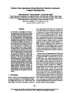
The file has 22,881 distinct words3 . We report CPU times. The problem settings of our experiments are not supported by the traditional algorithms, so we omitted any comparisons. It would be possible to use the traditional algorithms as filters for these problems, but this would require very large k 0 values, which would make the algorithms highly impractical. Fig. 1 (left) shows experiments for k = 0 for different k 0 values, for single pattern of length m = 12 words (note that M = m × b is about 70). The k 0 values are proportional to each word length in the pattern (i.e. the actual values were k 0 /100×|Pi |, where k 0 is reported in the plot). As shown both F ILTER of Sec. 3.5 and the exact matching algorithm BNDM of Sec. 3.4 are very fast. The filtering algorithm is compared against BP-DP-S EARCH for the same problem setting for k ≥ 0. The filter is clearly faster for small values of k, independent of k 0 . Fig. 2 shows timings for BP-DP-S EARCH for different r, k, and k 0 . The pattern lengths were m = 8 words. The time increases for larger number of patterns, but the result is still very efficient even for hundreds of patterns. The results could be still improved using the techniques described in Sec. 3.6 and Sec. 3.7.

5. Conclusions and future work We have considered approximate string matching in natural language using two level alphabet. Using the words of the text as the primary alphabet allows flexible approximate phrase matching, while using the characters of the words as a secondary alphabet allows approximate matching of the words themselves. We have obtained algorithms that perform the optimal number of word comparisons on average. As compared to traditional character level string matching, this new setting allows more complex search problems to be solved efficiently. The algorithms, however, are not complex, but simple to implement, and the experimental results show that they work well in practice. Our algorithms are based on indexing the text vocabulary, the word alphabet, in lazy manner, which allows straight-forward application of know results. Hence many other algorithms can be easily generalized as well, such as using regular expression matching in word level. On the other hand, as the matching algorithms and the vocabulary indexing are logically separated, it would be easy to allow more general matching relations between the words, such as adding a simple thesaurus on top of the index, allowing a pattern word to match its synonym word in text.

References [1] Baeza-Yates, R., Navarro, G.: Faster Approximate String Matching, Algorithmica, 23(2), 1999, 127–158. [2] Baeza-Yates, R., Navarro, G.: New and Faster Filters for Multiple Approximate String Matching, Random Structures and Algorithms (RSA), 20, 2002, 23–49. [3] Chang, W., Marr, T.: Approximate String Matching with Local Similarity, Proceedings of the 5th Annual Symposium on Combinatorial Pattern Matching (M. Crochemore, D. Gusfield, Eds.), number 807 in Lecture Notes in Computer Science, Springer-Verlag, Berlin, Asilomar, CA, 1994. [4] Crochemore, M., Czumaj, A., Ga¸sieniec, L., Jarominek, S., Lecroq, T., Plandowski, W., Rytter, W.: Speeding up two string matching algorithms, Algorithmica, 12(4/5), 1994, 247–267. 3

Without stemming. With stemming, only about 14,000.

0.055 0.05 0.045 0.04 0.035 0.03 0.025 0.02 0.015 0.01 0.005 0

Filter BNDM

time (s)

time (s)


0

5

10

15

20

25

30

35

0.5 0.45 0.4 0.35 0.3 0.25 0.2 0.15 0.1 0.05 0

40

465

DP k’ = 0 Filter k’ = 0 DP k’ = 20 Filter k’ = 20 DP k’ = 40 Filter k’ = 40

0

1

2

k’

3

4

k

Figure 1. Left: Times in seconds for searching a single pattern of length m = 12 words, for k 0 = 0% . . . 40%. Right: Times for k = 0 . . . 4.

0.35

0.8 k’ = 0 k’ = 20 k’ = 40

0.3

0.6 time (s)

time (s)

0.25 0.2 0.15

0.5 0.4 0.3

0.1

0.2

0.05

0.1

0

0 0

1

2 k

3

4

0

3.5 k’ = 0 k’ = 20 k’ = 40

3

time (s)

time (s)

2.5 2 1.5 1 0.5 0 0

k’ = 0 k’ = 20 k’ = 40

0.7

1

2 k

3

4

20 18 16 14 12 10 8 6 4 2 0

1

2 k

3

4

2 k

3

4

k’ = 0 k’ = 20 k’ = 40

0

1

Figure 2. Experimental results for BP-DP-S EARCH. From left to right, top to bottom: r = 1, r = 16, r = 64, and r = 256. In each case m = 8.

466


[5] Fredriksson, K.: Metric Indexes for Approximate String Matching in a Dictionary, Proceedings of the 11th International Symposium on String Processing and Information Retrieval (SPIRE’2004), LNCS 3246, Springer–Verlag, 2004. [6] Fredriksson, K., Navarro, G.: Average-Optimal Single and Multiple Approximate String Matching, ACM Journal of Experimental Algorithmics (JEA), 9(1.4), 2004. [7] Heaps, H. S.: Information retrieval: theoretical and computational aspects, Academic Press, New York, NY, 1978. [8] Hyyrö, H.: Explaining and Extending the Bit-parallel Approximate String Matching Algorithm of Myers, Technical Report A-2001-10, Department of Computer and Information Sciences, University of Tampere, Tampere, Finland, 2001. [9] Hyyrö, H., Fredriksson, K., Navarro, G.: Increased Bit-Parallelism for Approximate String Matching, Proc. 3rd Workshop on Efficient and Experimental Algorithms (WEA’04), LNCS 3059, 2004. [10] Hyyrö, H., Navarro, G.: Bit-parallel Witnesses and their Applications to Approximate String Matching, Algorithmica, 41(3), 2005, 203–231. [11] Moura, E., Navarro, G., Ziviani, N., Baeza-Yates, R.: Fast and Flexible Word Searching on Compressed Text, ACM Transactions on Information Systems (TOIS), 18(2), 2000, 113–139. [12] Myers, G.: A fast bit-vector algorithm for approximate string matching based on dynamic programming, J. Assoc. Comput. Mach., 46(3), 1999, 395–415. [13] Navarro, G.: Approximate Text Searching, Ph.D. Thesis, Department of Computer Science, University of Chile, December 1998. [14] Navarro, G., Raffinot, M.: A Bit-parallel approach to Suffix Automata: Fast Extended String Matching, Proceedings of the 9th Annual Symposium on Combinatorial Pattern Matching (CPM’98), LNCS v. 1448, Springer-Verlag, 1998. [15] Navarro, G., Raffinot, M.: Flexible Pattern Matching in Strings – Practical on-line search algorithms for texts and biological sequences, Cambridge University Press, 2002, ISBN 0-521-81307-7. 280 pages. [16] Sellers, P. H.: The theory and computation of evolutionary distances: Pattern recognition, J. Algorithms, 1(4), 1980, 359–373. [17] Shang, H., Merrett, T. H.: Tries for Approximate String Matching, Knowledge and Data Engineering, 8(4), 1996, 540–547. [18] Ukkonen, E.: Algorithms for approximate string matching, Inf. Control, 64(1–3), 1985, 100–118. [19] Yao, A. C.: The complexity of pattern matching for a random string, SIAM J. Comput., 8(3), 1979, 368–387. [20] Zipf, G.: Human Behaviour and the Principle of Least Effort, Addison-Wesley, 1949.