Department of Electrical and Computer Engineering. Purdue University, West .... If we assume seven task classes with the highest-reward tasks having reward.
On-line Scheduling via Sampling Hyeong Soo Chang, Robert Givan, and Edwin K. P. Chong Department of Electrical and Computer Engineering Purdue University, West Lafayette, IN 47907 (765) 494-{0643,9068,9143} {hyeong,givan,echong}@ecn.purdue.edu http://www.ece.purdue.edu/~{hyeong,givan,echong}
Abstract1 We consider the problem of scheduling an unknown sequence of tasks for a single server as the tasks arrive with the goal off maximizing the total weighted value of the tasks served before their deadline is reached. This problem is faced for example by schedulers in packet communication networks when packets have deadlines and rewards associated with them. We make the simplifying assumptions that every task takes the same fixed amount of time to serve, that every task arrives with the same initial latency to its deadline. We also assume that future task arrivals are stochastically described by a Hidden Markov Model (HMM). The resulting decision problem can be formally modelled as a Partially Observable Markov Decision Process (POMDP). We first present and analyze a new optimal off-line scheduling algorithm called Prescient Minloss scheduling for the problem just described, but with “prescient” foreknowledge of the future task arrivals. We then discuss heuristically adapting this off-line algorithm into an on-line algorithm by sampling possible future task sequences from the HMM. We discuss and empirically compare scheduling methods for this on-line problem, including previously proposed samplingbased POMDP solution methods. Our heuristic approach can be used to adapt any off-line scheduler into an on-line scheduler.
1. Introduction This work considers the problem of scheduling a sequence of tasks where the tasks are not all known to the scheduler at once, but rather arrive in an on-line fashion as scheduling proceeds. We use stochastic planning techniques to model and address the problem of selecting which task to serve in order to maximize the cumulative value of the tasks served over long time intervals (more precisely, we seek to maximize the discounted weighted number of tasks served, where each task carries a natural number weight indicating its value if served before its deadline). We make several simplifying assumptions in our first pass at this problem—these are primarily motivated by the need for analytical and algorithmic tractability, but also by correspondence to our motivating application of multiclass 1. This research is supported by the Defense Advanced Research Projects Agency under contract F19628-98-C-0051. The equipment for this work was provided in part by a grant from Intel Corporation. The views and conclusions contained in this document are those of the authors and should not be interpreted as representing the official policies, either expressed or implied, of the Defense Advanced Research Projects Agency or the U. S. Government.
packet-network scheduling. First, we assume that there are a finite number of different classes of tasks such that the reward associated with scheduling a task before its deadline is determined by the class into which it falls. These classes can be thought of as differing priorities (or pricings) of service. We assume that the task arrivals for each class are described stochastically by a Hidden Markov Model (HMM), one for each class,2 such that at most one task arrives per time step per class. In our problem setting there are no precedence constraints among the tasks, so that any task may be scheduled regardless of what other tasks have been scheduled. We assume that every task takes the same unit time to process, and finally, we assume that every task arrives with the same latency to its deadline: i.e., there is some fixed time interval d between the arrival time and deadline time that applies to every task. Even under all these simplifying assumptions this on-line scheduling task has no known optimal or approximately optimal solution that can be computed in reasonable time. The approach we take here is to model the problem as a discrete-time Partially Observable Markov Decision Process (a POMDP). POMDPs have recently been studied in the artificial intelligence literature as general models for planning in the face of uncertainty (Littman 1996). Optimal POMDP solution methods are known to be impractical in many cases even for small problems. Proposed approaches often rely on additional assumptions about the problem that are not present in this example (e.g., (Hansen, Barto, and Zilberstein 1996) relies on the presence of sensor actions that reveal the hidden state information). Queueing/scheduling problems such as the one we consider are most commonly formulated using continuous-time MDP or semi-MDP models (see for example (Stidham and Weber 1993)). For simplicity in explicating the connections to the AI POMDP literature we consider a discrete-time formulation here, but this work should generalize to continuous time. In this work we consider using sampling of possible futures to obtain an estimate of the expected value obtained by following each available action (i.e., scheduling each candidate task). Recent work reported in (Kearns, Mansour, and Ng 1999a), (Kearns, Mansour, and Ng 1999b) and in (McAllester and Singh 1999) has proposed sampling as a
2. In problems where the job arrival characteristics are not known (or are changing), an HMM model for each class can be inferred and updated over time using an expectation maximization (EM) algorithm.
means for evaluating or selecting a POMDP policy, respectively. Unfortunately, the approximately optimal sampling techniques presented in these previous papers appear to be completely impractical for reasonable parameter values of this problem. More specifically, if the sampling width and horizon for these algorithms are selected so that the approximation guarantees are non-trivial, then the amount of computation required cannot be carried out by any current computer hardware. As an example, suppose we use the sampling technique proposed in (McAllester and Singh 1999) and select the sampling parameters using the approximation bounds provided in that paper. If we assume seven task classes with the highest-reward tasks having reward 2000 and the lowest-reward tasks having reward 5, with discount factor 0.9, and if we require value estimates accurate enough to discriminate between a policy ρ that schedules a low-reward task at every time step and a policy ρ’ that schedules a high-reward task at every time step, then the method appears to require us to traverse a tree with branching factor of order 108 and depth greater than 60.3 In response to these practical difficulties, we have taken a different (and more heuristic) approach to using sampling to address this scheduling problem. This approach can be applied to any POMDP problem; however, it is clear that only problems with very particular structure will find this approach useful. Future work must be done to determine exactly what problem features are required to justify this approach—at this point, our evidence for the applicability of our approach to this problem is only empirical. Our approach is to begin by designing a policy selection method for the related off-line scheduling problem—i.e., the problem where the future task arrivals are known. For this problem, we are able to give an algorithm that computes an optimal schedule, and this paper presents that algorithm and argues its optimality. It is important to note that in this off-line scheduling problem, tasks cannot be scheduled before they are slated to arrive—in other words, the arrival sequence is still important and we are not simply scheduling a set of tasks. This off-line algorithm can then be used to get a heuristic estimate of the value obtainable from a given POMDP belief state by using sampling, as follows. Using sampling, we can compute the expected value obtained from any belief state by the off-line algorithm over the problem-specified distribution of job arrival sequences: we simply sample several task arrival sequences from the HMM and compute the mean performance of the off-line scheduler on those sequences. This corresponds to measuring the expected performance of a “prescient” version of the off-line algorithm—one that can see the future arrival sequence. There is no guarantee that this will correspond to the performance of any “non-prescient” scheduler. This sampling-based value estimate can then be used to estimate the Q-value for each possible scheduling choice and choose a task to schedule. To do this in practice also requires maintaining and up3. The high branching factor derives from the high sampling width required for reasonable accuracy.
dating a current POMDP belief state after each action is taken, to use as the starting point for sampling. To generalize this approach to an arbitrary POMDP (which will often perform quite poorly, we believe), we must view the off-line algorithm as a means of taking a POMDP belief state and a fixed random number sequence and returning the optimal finite-horizon value obtainable from the belief state, assuming that any stochastic choices encountered are made in sequence according to the fixed random number sequence. (In our problem, the only stochasticity in the problem comes from the uncertain future task arrivals, and so presciently knowing the future task sequence is equivalent to knowing how each stochastic choice will be resolved, i.e., knowing the random number sequence used in task sequence generation.) Given a similar off-line algorithm for an arbitrary POMDP, we can then estimate the expected value of acting “presciently optimal” in that POMDP, and base our action choice on that estimate. It cannot be overemphasized that for many POMDP problems this will yield very poor performance (we show an example later). The usefulness of this technique clearly relies on special characteristics present in scheduling-derived POMDPs (and perhaps other POMDPs—we have not yet been able to characterize the class of POMDPs where this technique would apply). We have implemented an on-line scheduling system based on these ideas, and compared its performance with two approaches that ignore future-arriving tasks until they arrive, and with the more principled sampling approach described in (McAllester and Singh 1999) with sampling parameters set small enough to make the sampling practically computable (thus losing any useful approximation guarantees). Our system performs favorably with respect to these other approaches. A key approach we have not yet compared to our work empirically is the approach presented in (Crites and Barto 1996) for elevator scheduling. This approach analyzes an MDP problem formulation using function approximation to cope with the large state space and off-line Q-learning to find an effective policy. While it is not immediately clear how to apply this approach to a POMDP setting, we plan to eventually compare our approach to a Q-learning based approach (perhaps learning for the continuous “informationstate” MDP form of the POMDP). This alternative still requires substantial off-line training in contrast to our approach, but the resulting policy is more clearly implementable in an on-line scheduler (no sampling to be done). In the remainder of this paper, we formally define in turn: the on-line scheduling task we are addressing, the POMDP formalism we are using to represent the decision-making task, the off-line scheduling algorithm we have designed (including its optimality proof), and the sampling adaptation of this off-line algorithm. We then give empirical results for some particular instances of this task comparing our algorithm to other approaches.
2. On-line Task Scheduling with Deadlines We assume that time t is discrete, i.e., t ∈ {0,1,2,...}, and
that each task takes exactly one time step to be served. We assume there are m > 1 different classes of tasks involved in the problem, with positive real reward λi > 0 associated with each class i ∈{1, ..., m}. We assume without loss of generality that for i < j, λi > λj, i.e., that the classes are arranged in order of descending reward. For each task class i, we assume some unknown arrival sequence given by Ai(t) ∈ {0,1} as t varies in T. In other words, a task arrives at time t in class i if and only if Ai(t) is 1. Let A(t) be the m-tuple of arrivals for the different m classes , so that A constitutes a complete description of the arrival sequence for all classes, and is called a task arrival pattern. Note that for simplicity we do not allow multiple tasks in the same class to arrive at the same time, and tasks arriving at different times or in different classes are assumed distinct from one another. When needed, we will refer to the task arriving in class i at time t (if any) as task pi,t. Every task is assumed to have a “builtin” arrival time, and the same deadline d relative to its arrival time—i.e., task pi,t must be served/scheduled at a time t’ in the range t ≤ t’ < (t + d) or it is considered lost. We refer to the latest time a task pi,t can be scheduled (t+d–1) as the deadline for the task, denoted deadline(pi,t). Task pi,t is said to be live for times in this range only. A task pi,t is said to be earlier than a task pi’,t’ if t < t’. Definition 1: A schedule π(t) is a mapping from times t ∈ T to classes {1, ..., m} or “idle” giving the class4 of task served at time t. The schedule πt is the schedule π restricted to times 0, ..., t–1 and “idle” otherwise, and is called a prefix schedule, so that π0 is the completely “idle” schedule. We say that π schedules a task pi,t at time t’ if and only if π(t’) is i, Ai(t) is 1, pi,t is live at time t’, and all earlier tasks pi,t’’ that are live at time t’ are scheduled by πt’. A task is unscheduled by π if it is not scheduled by π at any time. The schedule π is well-formed for arrival pattern A if for all t, π(t) is “idle” when no task is actually scheduled (i.e., π(t) is never a class with no live task unscheduled by πt). In analyzing our algorithms, we also need schedules that specify exactly which tasks to serve at each point in time: Definition 2: A task mapping is a one-to-one partial mapping σ from times to tasks such that σ(t) = p implies that p is live at time t. The schedule πσ induced by σ is the schedule that serves class i at time t if and only if σ(t) is in class i, and is “idle” if σ(t) is undefined. For each class i, the schedule induced by σ schedules the same number of class i tasks as appear in the range of σ. Every wellformed schedule π is πσ for some task mapping σ. Definition 3: A scheduling policy S(πt, A), is a mapping from a prefix schedule πt and arrival pattern A to a class i to be scheduled next. Policy S is said to generate the schedule π on arrivals A if π(t) is equal to S(πt, A) for all 4. A schedule can select only the class and not the actual task at each time step because we always serve the earliest unexpired task of a given class—this can readily be seen to preclude only “dominated” schedules.
times t. By abuse of notation, this schedule is written S(A). A scheduling policy S is said to be work-conserving if every schedule π generated by S has a task scheduled at every time t for which there is a live task not already scheduled by π at any previous time. Policy S is said to be causal, or on-line if its output on prefix policies πt does not depend on the values Ai(t’) for times t’ > t; otherwise, S is said to be off-line. Definition 4: The γ-discounted weighted task loss Wπ incurred by a schedule π is the sum for all arriving tasks pi,t unscheduled by π of the class reward λi lost by not serving the task pi,t times the discount factor γ raised to the 1+deadline(pi,t) power5. We seek a policy minimizing γ-discounted weighted task loss for γ arbitrarily close to one. Definition 5: A scheduling policy S dominates a policy S’ if there is some discount factor γ such that for every γ’>γ and every arrival pattern A, WS(A) ≤ WS’(A). We would ideally like to find an on-line scheduling policy S that dominates all other on-line scheduling policies. Unfortunately, it is not hard to show that in general there is no such policy (e.g., see (Chang et al. 2000)). For any candidate on-line policy, we can find an arrival pattern and alternative on-line policy such that the alternative policy outperforms the candidate policy on the selected pattern by incurring less weighted task loss. Therefore, it is necessary to consider a prior distribution over arrival patterns in order to define a desired optimal policy. Definition 6: A scheduling policy S is said to be optimal for a given probability distribution P over arrival patterns A if for every alternative policy S’ the expected value over all A of WS’(A) exceeds the expected value of WS(A). It follows from the theory of POMDPs that for any distribution P over arrival patterns and any finite horizon, there must exist an optimal scheduling policy S; however, computing this policy for an arbitrary P and large horizon can be extremely difficult and is in general intractable. We investigate known techniques for approximating the optimal policy and compare them to our heuristic technique. First, we must discuss our model for the probability distribution P over arrival patterns. Modeling Task Arrival Distributions. Our approach to modeling distributions over arrival patterns is to give a hidden Markov model (an HMM) for each class i that generates the arrival pattern Ai for that class. An HMM is a tuple where Q is a finite set of task-generation states, T gives the next state probability distribution for each state in Q, Λ is a mapping from Q to probabilities giving the probability of a task arrival per time step for each state, and Π is a distribution over Q representing the uncer5. Note: discounting is introduced here for consistency with the POMDP formalism we adopt later and the AI literature on POMDPs—however, the nature of the scheduling problem makes discounting inessential and an alternative formulation in terms of rolling finite-horizon windows is also acceptable. Our general techniques do apply to problems where the discount factor is important.
tain initial state of the HMM. A (hidden) state sequence is generated by the HMM with probability given by Π(q1) times the product over all i in 1, ..., k–1 of T(qi, qi+1). The probability that the state sequence will generate a given arrival pattern where each ai ∈{0,1} is given by the product over all i in 1, ..., k of [ai Λ(qi) + (1–ai) (1–Λ(qi))]. Finally, the overall (hidden state sequence independent) probability that the HMM will generate a given arrival pattern is the sum over all state sequences of the probability of the state sequence times the probability that the state sequence will generate the arrival pattern. Standard techniques generalize these definitions to infinite length sequences. HMM models can generate a wide range of different bursty and non-bursty arrival patterns of arbitrary complexity depending on the size of the state space Q (Fischer and Meier-Hellstern 1992)(Michiel and Laevens 1997). We note that for applications where the task arrival pattern is not known, or is changing over time, well-known variants of the expectation-maximization (EM) algorithm can be used to infer an HMM heuristically describing the pattern from observations of the pattern over time (Rabiner 1989). For the remainder of this work we assume that an accurate HMM model for the distribution P is provided. POMDP Models for On-line Scheduling. The optimization problem involved in selecting a scheduling policy for a specific HMM describing the arrival patterns can be formulated as a partially observable Markov decision process (POMDP). Here we briefly review POMDPs and relate them to our problem—for a more substantial introduction please see (Littman 1996) or (Kaelbling, Littman, and Cassandra 1998). A POMDP is a 7-tuple where Q is a set of system states, I is a set of available actions, T gives the next-state probability distribution for each state and action, R gives the reward obtained for taking an action at a state, O is a set of possible observations, Z gives a distribution over observations for each state, and Π is a distribution over Q representing our uncertainty about the initial system state. If the actual current state is q and we take action a, we receive a reward of R(q, a), and the probability that the state will transition to q’ is T(q, a, q’). The probability that the state sequence is generated in response to the action sequence is Π(q1) times the product over all i in 1, ..., k–1 of T(qi, ai, qi+1). The tuple (without the “observation” components O and Z) specifies a Markov decision process (MDP). A policy π for the MDP is a mapping from Q to I specifying the action to take at each state. For a given policy π, we define the infinite-horizon discounted reward t starting at state q as lim t → ∞ ( E [ Σ i = 0 ( γ i ⋅ r i ) ] ) , where ri is a random variable representing the reward received at time i and γ is a positive real-number discount factor less than 1. Under general conditions, there is an optimal policy that maximizes the infinite-horizon discounted reward. The POMDP introduces the complication that our plan cannot be a mapping from states to actions, because we do not have access to the states. Instead, we have to work with the observation sequence—if
the underlying state is q, we make an observation o with probability Z(q, o). An optimal policy for a POMDP can be defined by converting the POMDP into the equivalent “information-state MDP” (ISMDP) over “belief states”. A belief state b is a probability distribution over Q representing the probability that the underlying MDP is in each state. Starting with the initial belief state Π of the POMDP, a straightforward application of Bayes rule can be used to update the belief state at each state transition as a function of the action taken and the observation seen. This “belief-state update rule” essentially defines the transition probabilities for the related ISMDP, where the state space is the possible belief states. In particular, this defines transition probability function T’, defined in terms of T and Z, such that given a belief state b and an action a, T’(b, a, b’) is the probability that the next belief state is b’. Similarly, the reward function R’ for the belief MDP can be defined in terms of T, Z, and R. A policy for the POMDP/ISMDP can then be specified as a map from belief states to actions. The infinite-horizon discounted reward starting from any initial belief state b is therefore well-defined, the optimal value of which is called the value function, denoted V*(b). Defining the Q-function for action a by Qa(b) = R’(b, a) + γ Σb’[T’(b, a, b’) V*(b’)], it can be shown that the optimal policy for the POMDP is given by π’(b) = argmaxa Qa(b, a). We can now describe how to formulate our scheduling problem as a POMDP . Let be the HMM for the arrivals of class i ∈ {1, ..., m}. The state space Q of the POMDP is Q = Q 1 × ... × Q m × {0,1}m× d, where the last factor represents the currently arrived unserved tasks, indexed by class and time remaining to deadline—given a particular state, this component of the state is called the buffer of the state. The set of actions is I = {1, ..., m}, where action a = i means that we serve the earliest live unserved task in class i. The state transition function T is defined in the obvious manner representing underlying stochastic transitions in each of the arrival HMMs, and the change in the buffer by adding new tasks generated stochastically by the arrival HMMs as well as the expiry of unserved tasks and the removal of the task served by the action selected. The reward function R is defined as R(q, a) = λa. The set of observations O is given by O = {0, 1}m, representing the observed arrival or nonarrival of a task in each class. The probability Z(q, o) of making observation o at state q is either 1 or 0 according to whether o precisely describes the final column of the buffer in q. An alternative R function can easily be designed to describe the equivalent problem of minimizing weighted loss (here we have described maximizing weighted throughput). We select a discount factor γ arbitrarily close to one because the nature of the scheduling problem makes discounting inessential— good policies must serve as much weight early as possible with or without discounting. Our actual finite-horizon sampling algorithms will treat the discount factor as equal to one.
3. Non-sampling On-line Policies In this section we describe three basic on-line scheduling
policies that use no information about the distribution of arrival patterns to provide a baseline for comparison and to provide a starting point for defining our sampling policy. First, two very simple policies: one that ignores deadlines and another that ignores task class. Definition 7: The static priority (SP) policy is the policy SP such that SP(πt, A) is the highest reward class that has a task unscheduled by πt that is live at time t (breaking ties by serving the earlier arriving task) Definition 8: The earliest deadline first (EDF) policy is the policy EDF such that EDF(πt, A) is the class with the earliest-expiring task unscheduled by πt that is live at time t (breaking ties by serving the higher class task). Next, we consider policies that act at each time step to minimize loss under the assumption that no further tasks will arrive, which we call “current-minloss policies.” We say that a task arrival pattern A is finite if Ai(t’) is zero for all i and all t’ ≥ t for some t called the horizon of A. We say that a schedule π starts at time t if π(t’) = “idle” for all t’ < t. Also, for any set of tasks K, we can construct an arrival pattern AK corresponding to the arrivals of those tasks at their respective arrival times, and no other arrivals. Definition 9: A minloss schedule πA for a finite arrival pattern A is a schedule that achieves lower weighted loss than any other schedule for A (at the horizon time of A plus d). A minloss schedule for A starting at time t (πAt ) is a schedule starting at time t that achieves lower weighted loss on A than any other such schedule. If the tasks in A have all arrived at time t, we call this a current-minloss (CM) schedule starting at time t. Definition 10: A current-minloss (CM) policy is a policy CM that always schedules a class that is scheduled by at least one current-minloss schedule for the currently live unscheduled tasks (i.e., ignoring future arrivals). More formally, if CM(πt , A) is the class i then there must be some CM schedule πAt’ starting at time t for arrival pattern A’ = A K where K is the set of live tasks at time t that are unscheduled by πt , such that πtA’ (t) = i. It is possible to give on-line CM policies. Constructing a CM policy involves finding at each time t a CM schedule starting at t for the live unscheduled tasks at time t. We give in Figure 1 the pseudo-code for an implementation of a particular on-line CM scheduler. The problem at each time t is a special case of the general job sequencing problem solved by Sahni (Sahni 1976). Sahni’s approach specializes to a O(d 2) time complexity CM policy for our problem—the CM policy we sketch in Figure 1 can be implemented to obtain a tighter O(d+m) performance because it is optimized for our problem assumptions.6 Our algorithm greedily schedules each task in the latest available time slot for which the task is live, considering 6. Implementing the sketched CM policy directly from this pseudo-code will also give O(d 2) time complexity, however the line that computes slot can be optimized by using union-find on sets of times. Also, the O(d+m) bound stated omits an inverse Ackerman’s function factor from the union-find algorithm.
tasks from high-reward classes first, and within each class later deadline tasks before earlier deadline tasks. The pseudo-code in Figure 1 also achieves a CM schedule in this manner in Step 1, and then goes on in Step 2 to improve the schedule for use in “non-current” contexts (i.e., when future arrivals are expected) by reorganizing the schedule to serve the highest possible reward task first without losing the CM property. For the remainder of this paper we refer to this algorithm as the CM policy. Let plan be a mapping from times t, ..., t+d–1 to tasks or “idle”, initialized at all time steps to “idle”. Step 1: Generate a current-minloss task schedule for class = 1 to m // highest weight class first for task in class, latest-arrived to earliest-arrived slot = the largest j ≤ deadline(task) such that plan[j]==“idle”; if such slot exists, then plan[slot] = task; endfor endfor Step 2: Select a class to serve next using plan cut = the smallest time t’ such that forall t’’≤ t’, deadline(plan[t’’]) ≤ t’ // tasks up to plan[cut] can all be served no matter // which task is actually scheduled first: Select the highest-reward class of plan[t],..., plan[cut] Figure 1: Code sketch for our CM policy Theorem 1: Figure 1, Step 1 defines a CM policy. Proof: We say that a task mapping σ is a “CM mapping” if πσ is a CM schedule, and we call a partial mapping σ “acceptable” if it can be extended to a CM mapping. The empty mapping is “acceptable” in this sense. Consider an acceptable mapping σ. Let i be the class of the highestreward arriving task that can be added to σ to get another task mapping. Let p be the latest arriving task in class i not already in the range of σ. Let σ’ be the mapping that extends σ by scheduling p at the latest time t’ such that p is live at t’. (This is exactly the extension to plan that is carried out by the for loops of step 1 of the algorithm.) We argue that σ’ is acceptable. By definition, some extension σ’’ of σ is a CM mapping. σ’’ must schedule some class i task not scheduled by σ, or modifying σ’’ by setting σ’’(t’) to be p would produce a mapping that schedules more class weight than πσ’’, contradicting the choice of σ’’ as a CM mapping. But if σ’’ schedules any class i task p’’ not scheduled by σ at any time t’’, then t’’ must be less than t’, given the way we chose t’. But then σ’’ can be modified into a CM-mapping extending σ’ by swapping σ(t’) and σ(t’’), and then replacing p’’ by p as the value of σ(t’). Q.E.D.
Unlike Sahni’s algorithm, our CM policy is designed for use in an on-line setting (hence Step 2 in the code sketch). Thus unlike Sahni, we have analyzed the policy’s on-line performance. We can show the following two modest assertions hold regarding this performance (see also (Hajek and Seri 1998) for general related results). Theorem 2: The CM policy strictly dominates the EDF policy (i.e., CM wins/ties regardless of arrival pattern). Theorem 3: The CM policy is work-conserving and (unweighted) throughput optimal (i.e., for any arrival pattern CM generates a schedule that serves the maximum number of tasks).
4. Off-line Scheduling for Minimum Loss We consider the problem of scheduling a finite arrival pattern A for minloss in an off-line manner, i.e., as though we know ahead of time in what pattern the tasks will arrive. This problem corresponds to a standard job sequencing problem where each job has both a deadline and a “ready time” (the arrival time, before which the job cannot be scheduled) (Kise, Ibaraki, and Mine 1978), (Lawler 1964), (Lawler 1976), (Moore 1968), (Villareal and Bulfin 1983). We have found no previous work7 combining deadlines, ready times, and the weighted task optimality criterion—we give a polynomial-time algorithm addressing all these factors. The problem is known NP-hard without our assumption that each task has the same fixed deadline d at its arrival and the same fixed processing time (i.e., the problem is NP-hard with arbitrary task ready and deadline times or task processing times) (Lenstra 1977). The constraint that a task cannot be scheduled prior to its arrival adds complexity to the minloss scheduling problem. Neither of the observations used in Section 3 in designing the CM policy holds for this richer problem. Because the problem involves apparent foreknowledge of the arrival pattern, we refer to algorithms addressing it as “prescient”. Definition 11: A minloss policy is an (off-line) policy that generates a minloss schedule for any finite arrival pattern. We present and argue correctness for a particular minloss policy based on an elaboration of the approach taken in CM. We schedule tasks greedily from the highest-reward class to the lowest, and within a class from latest arriving to earliest arriving. As in CM, we start by scheduling tasks for service at the latest open schedule slot not after the task deadline. However, unlike in CM, we cannot be guaranteed that this initial task placement in the schedule can be extended to a full minloss schedule. The initial placement may be revised by the algorithm as additional tasks are scheduled. Similarly, we cannot drop a task (i.e., not add it 7. It has since come to our attention that a symmetric variant of this algorithm (reversing time and swapping ready/deadline times) has been published in the performance evaluation literature for a different purpose—providing an upper bound on performance to use in evaluating scheduling algorithms. Our optimality proof is different and apparently more complete. See (Peha 1995).
to the schedule) if there is no idle slot in the schedule during the task’s live period—we must consider moving other tasks that are scheduled during that period to make room. This complexity is a result of having to consider varying task arrival times in addition to deadlines (unlike in the CM scheduling problem where all the tasks have currently already arrived). To handle this complexity, we introduce a new concept: Definition 12: Given a task mapping σ and times t and t’ with t < t’, a shuffle on σ moving time t to time t’ is a permutation R of a finite set BR of times including t and t’ such that for each time t’’ in BR (other than t),
• R(t’’) < t’’, • if defined, σ(t’’) is a task that is live at time R(t’’), and • R(t) = t’. The result of applying a shuffle R to σ is a new task mapping (written R(σ) by abuse of notation) defined to equal σ except that for each t’’ in BR, [R(σ)](R(t’’)) is set to σ(t’’). We can now describe the basis of our PM algorithm. We construct a task mapping incrementally, starting from the empty task mapping (undefined everywhere), and considering tasks for addition to the mapping greedily from the highest-reward class to the lowest, and within a class from latest arriving task to earliest arriving. Once a task is considered and rejected that task never needs to be considered again. Given a partial task mapping σ and a task p to be considered for addition to σ, we let t be the latest time ≤ deadline(p) such that σ(t) is undefined. We then admit p to σ if there exists a time t’ when p is live and a shuffle R on σ moving time t to time t’. If there is such a shuffle R and time t’, we update σ to R(σ) and then set σ(t’) to p. A key and nontrivial property of this algorithm is that the set of scheduled tasks after any task is considered does not depend on the choices of shuffles made up to that point (see proof below). We give a code sketch for an O(H 2+m) minloss scheduler in Figure 2, for sampling horizon H. We henceforth refer to this policy as the “prescient minloss” (PM) policy. We start our analysis of this algorithm by proving a key lemma, mentioned above. The lemma depends critically on the following definition of a function slack that maps task mappings to vectors of numbers. Definition 13: Given a partial task mapping σ defined on times {0, ..., H}, the slack of σ is a vector where si gives the number of tasks scheduled by σ at times ≥ i that are live at time i–1. More formally, si gives the cardinality of the set {t | t ≥ i and σ(t) is defined and is live at time i–1}. (s0 is always zero.) Lemma 1: The sequence of tasks admitted to the task mapping σ (plan in the code sketch) does not depend on the choices of shuffles made in the calls to find-shuffle. Proof: The lemma follows from these observations:
Let plan be a mapping from times 0, ..., H to tasks or “idle”, initialized at all time steps to “idle”. Step 1: Generate a prescient-minloss task schedule for class = 1 to m // highest weight class first for task in class, latest-arrived to earliest-arrived slot = the largest j ≤ deadline(task) such that plan[j]==“idle”; shuffle = find-shuffle(arrival-time(task), slot) if such slot and shuffle exist, then {apply shuffle to plan; plan[slot] = task} endfor endfor // Finding a shuffle // ------from any time t before arrival-time, to empty-time find-shuffle (arrival-time, empty-time) { Let shuffle be a sequence of times t1, ..., tj representing the permutation t1→ ...→ tj→ t1. Initialize shuffle to the unit sequence of one time empty-time. last-added = empty-time; found = true; while (arrival-time > last-added) and found found = false; for offset = 1 to d–1 if plan[last-added–offset] is live at time last-added then {found = true; last-added –= offset; add last-added to shuffle at seq. start; break the for loop} endfor endwhile if found then return(shuffle); else return(fail); } // end of find-shuffle Step 2: As given for CM in Figure 1. Figure 2: Code sketch for our PM policy a. For any shuffle R on σ moving a time emptytime to a time when the newly admitted task p is live, the slack and idle times of the new task mapping resulting from applying R to σ and adding p depends only p and the slack and idle times of σ, and not on any other details of σ or on the shuffle used. b. The existence of a shuffle allowing p to be added to σ depends only on p and the slack of σ, but not on any other details of σ. Theorem 4: The PM policy in Figure 2 is a minloss policy.
Proof: (sketch) The proof of this theorem using Lemma 1 is non-trivial, but similar to the proof of Theorem 1; a complete proof will be provided in the full version of this paper. To finish the proof of Theorem 4 requires showing (as we did in proving Theorem 1) that the scheduler would never profit from passing up scheduling a late-arriving high-reward task in hopes of scheduling some earlierarriving task of the same class (or some lower-reward task) instead. This fact essentially follows from the fact that passing up the one task will never allow the scheduling of two other tasks in its place—proving this involves generalizing the proof of Theorem 1 to handle the presence of shuffles, but space does not allow us to present the proof here. Q.E.D.
5. Extending Off-line Scheduling by Sampling The off-line PM policy just described would be the ideal scheduler to apply but for the fact that in an on-line setting we do not have access to the future arrival sequence. Instead, we have the stochastic model generating this sequence in the form of an HMM for each class, constituting a POMDP problem (equivalent to a related ISMDP). We have investigated sampling from the ISMDP in a principled manner using the techniques described by McAllester and Singh (McAllester and Singh 1999)8. The approximation bounds given in that work require a computationally intractable amount of sampling to be done in order to get a useful guarantee of accuracy. However, the techniques described can be used with much smaller amounts of sampling giving up any approximation guarantee. We have implemented and tested this approach, and our preliminary results indicate that the resulting policy is generally inferior to the SP policy defined in Definition 7. Augmenting the policy by using our CM policy to estimate values at the horizon improves performance but the resulting policy does not outperform CM itself.9 These poor results are no doubt due to low sampling width and short horizon. (see below) In response to this poor performance, we have considered an alternative, heuristic sampling approach. This approach is based on the following observations about the optimal value function for a POMDP. The V* value function is defined in an “expectimax” fashion—being the max over all actions of the expected value of V* at the next state (which itself is the max over all actions of the expected value of V*
8. We note that a critical feature of the techniques in (McAllester and Singh 1999) is the compact approximate representation of the POMDP belief state. This compact approximation is not needed in our problem because we have a natural factoring of the belief state into factored observable state (the buffer contents) and unobservable state (the hidden state of the task arrival process). Although our overall statespace is very large, the arrival process state space can reasonably be assumed to be modest in size, so we can represent a belief state easily. 9. Achieving even this performance requires modifying the original techniques by using the same sampled arrival patterns for evaluating each action at a given choice point. Sampling anew for each action evaluation increases the variance in the value estimates and destroys performance. This use of common samples is also important to our method and derives from work in discrete-event systems on common random numbers simulation in perturbation analysis.(Ho and Cao 1991).
at the second next state, etc.). When the state space is small, dynamic programming can collapse the resulting expectimax tree.10 However, with the very large state spaces widely encountered in AI problems, dynamic programming is of very limited use. The sampling technique of McAllester and Singh is the principled way to sample from such an expectimax tree, but is also too expensive in this case. We consider here the heuristic approach of rearranging the tree so that all the expectation nodes come above all the max nodes in order to get an upper bound on the true value (formalized below), starting with a finite horizon tree11. For a general POMDP (even a fully observable one) this approach may not yield useful results, as it resembles assuming we know what each action will do before deciding whether to take it—this essentially allows the value estimate to be based upon a careful “lucky” walk through a minefield. In particular, optimal POMDP and MDP policies need to avoid taking actions that have significant chance of leading to very bad states, even if those actions also have a chance of leading to good states. Taking all expectation outside of the maximization steps effectively computes a value estimate based on a non-stationary policy that takes a given action only when it will “luckily” have a desired result. This can result in an action appearing beneficial when the Q-function value for the action is very poor. For an example, this approach will choose to walk through a minefield to avoid a safe tollbooth if there are “wait” and “walk” actions such that the “wait” action is completely safe and the “walk” action has some probability of killing you (when in the minefield) and some probability of safety. However, for some POMDPs12, including the scheduling POMDP we are addressing here, it appears that this unprincipled approach yields a reasonable approximation of the true relative value of each action (the Q-functions). “Knowing” the future in the sense of this approach leads to erring only on the side of overestimating state value (in any POMDP). It appears that for our POMDP this results in a similar amount of overestimation for the different states reachable by different actions from a single source state— this is expected because these single-step reachable states are all very similar. All the uncertainty is coming from the arrival pattern distribution, and that applies equally to every action. We now describe this approach more concretely for our problem and then present a brief formal analysis. For our problem, we start by using the POMDP belief state update rule to maintain a belief state over time (note
10. An expectimax tree is a tree where odd-depth nodes are labelled with “expectation” and even-depth nodes are labelled with “max”. If the leaves are labelled with numbers, a value can be computed recursively at every node by performing the function given by the node label on the values of the children of the node. 11. We note that Hauskrecht has considered a similar rearrangement of this expectimax tree independently for a quite different but related purpose. See p. 86 of (Hauskrecht 1997). 12. One candidate class is the class of exogenous control problems—problems where the action choice has no effect on the source of uncertainty. However, it is not clear how to define this class of problems formally, as it seems any POMDP can be viewed this way by thinking of all randomness as coming from a stream of random numbers generated independently of the control applied.
that the states of the arrival-generating HMMs are not directly observable). We can then select an action by estimating the Qa-function at the current belief state, for each action a. To do this, we apply each action a in turn to the current belief state, and use our heuristic sampling technique to estimate the V* value at the resulting belief state q. We assume the scheduler knows the HMM models from which arrivals are drawn, which can then be used to generate the samples of possible future arrivals. The V*(q) estimate is derived by averaging over n samples S of future arrivals out to some horizon H, and using the PM scheduling policy to compute the exact minloss schedule value achieved from state q on encountering sample S with prescient foreknowledge. We call this policy the Sampled PM policy (SPM) (no relation to the SP policy of Definition 7). The V*-value estimate given by the SPM algorithm does not provide a principled estimate of the finite horizon V* function for an ISMDP. Instead, we are estimating a function we have named the J-function, defined below, that upper bounds the V* function. First, we state the finite horizon undiscounted total reward VH* definition for comparison. We set V*0 (q) = 0, and V*H (q) = maxa R(q,a) + E T(q,a,q’)[V*H–1 (q’)].
(1)
These equations can readily be seen to describe an expectimax tree where the max nodes are each computing V*h (q’) for some state q’ and some horizon h between 1 and H. This is the tree that a principled sampling algorithm must approximate by sampling after each action choice-point. An * (q) is as follows. equivalent definition for VH V H* (q) = max 〈 π
1,
…, π H 〉 E [
Σi = 0 r i ] H
(2)
where ranges over sequences of policies (i.e., a non-stationary policy), and the random variable ri gives the reward at time i given that for each time i the policy πi is followed. For either V*H equation, sampling to estimate the expectation must be conducted inside an exponentially branching choice of a sequence of actions/policies, if we are to estimate VH* (q) in a principled manner. We do not have any answer for this difficulty for general POMDP problems; however, for problems with special structure like the scheduling problem described here, we can sample as described for the SPM algorithm above. In this case, we are instead computing the following equation, where the maximization is now inside the expectation. J H (q) =
H E max 〈 π1, …, πH〉 Σ i = 0 r i
=
H E max 〈 a1, …, aH〉 Σ i = 0 r i
(3)
Since the term inside the expectation is computed by PM, we can compute JH by sampling and running PM. JH (q) can informally be seen to upper bound VH* (q) by observing that the maximization is done for each stochastic future rather than once for all possible futures.
6. Empirical Results
10000
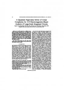
As with many AI problem domains (for example, propositional satisfiability), randomly selected problems from this scheduling domain are typically too easy (for satisfiability, such problems are easily seen to be satisfiable or easily seen to be unsatisfiable). In scheduling, this problem manifests itself in the form of arrival patterns that are easily scheduled for virtually no loss, and arrival patterns that are apparently impossible to schedule without heavy weighted loss (in both cases, it is typical that blindly serving the highest class available performs as well as possible). Difficult scheduling problems are typified by arrival patterns that are close to being schedulable with no weighted loss, but that must experience some substantial weighted loss. We have conducted experiments by selecting HMM models for the arrival distributions at random from a single distribution over HMMs. There is not room in this work (space- or time-wise) for an extensive study determining which distributions over HMM arrival descriptions yield hard problems and why, but this is a good topic for future work. At this point we have made some guided ad-hoc choices (see below) in selecting the distribution over HMMs from which to conduct our experiments. Given the selected distribution over HMMs, we have tested our SPM and CM algorithms, along with SP and EDF, against six different specific HMM arrival descriptions drawn from the distribution. For each such arrival description, we ran each scheduling policy for 2 × 10⁵ time steps and measured the weighted loss achieved by each policy over time. We show one such plot as an example in Figure 3. To summarize all the plots effectively, we have calculated the weighted-loss rate for each policy against each arrival pattern—this is the slope of the weighted loss versus time plot. Weighted-loss rates for the four algorithms versus each of the 6 arrival patterns are shown in Table 1. We give a brief description of an ad-hoc choice involved in selecting our distribution over HMMs. All of the problems we consider involve 7 classes of tasks. We select an HMM for each class, chosen from the same distribution. We selected the HMM state space of size 3 arbitrarily for these examples, resulting in a total hidden state space of 37 states. We selected the 7 class weights 13 as 2000, 1000, 800, 600, 20, 10, 5. Given the small state space for each HMM, we deliberately arrange the states in a directed cycle to ensure that there is interesting dynamic structure to be modeled by the POMDP belief state update (we do this by setting the non-cyclic transition probabilities to zero). Similarly, we select the self transition probability for each state uniformly in the interval [0.9, 1.0] in order that state transitions are seldom enough that observations as to what state is active can accumulate. We select the arrival generation probability at each state so that one state is “low traffic” (uniform in [0, 0.01]), one state is “medium traffic” (uniform in [0.2, 0.5]), and one state is “high traffic” (in [0.7, 1.0]). Finally, after selecting the HMMs for each of the
9000
13. We have not found performance to be very sensitive to class weight choices, as long as they are not extremely similar or dissimilar.
EDF SP CM SPM
Cumulative weighted loss
8000 7000 6000 5000 4000 3000 2000 1000 0 0
2
4
6
8
10 Time
12
14
16
18 4
x 10
Figure 3: Example weighted-loss plots for a single arrival pattern. HMM#: EDF SP CM SPM
1 0.33 0.27 0.019 0.013
2 5.63 3.93 1.02 0.84
3 0.54 0.26 0.051 0.044
4 1.61 1.76 0.26 0.22
5 0.51 0.32 0.039 0.025
6 2.17 1.27 0.34 0.30
Mean 1.80 1.30 0.29 0.24
Table 1: Weighted-loss rates for all HMMs tested. seven classes, we generate a large traffic sample and use it to normalize the arrival generation probabilities for each class so that arrivals are roughly equally likely in high-reward (classes 1&2), medium-reward (classes 3&4), and low-reward (classes 5–7), and so that overall arrivals occur at about 1.5 tasks per time unit to create a scheduling problem that is suitably saturated to be difficult. Even with these assumptions, a very broad range of arrival pattern HMMs can be generated. Without some assumptions like those we made here, we have found (in a very limited survey) that the arrival characterization given by the HMMs generated is typically too weak to allow any effective inference based on projection into the future. As a result, CM and SPM typically perform very similarly, and SP often performs nearly as well. The precise HMMs used are available on request. Examination of the weighted-loss rates shown in Table 1 reveals that the basic CM policy dramatically outperformed EDF and SP on all the arrival patterns, unsurprisingly. The heuristic sampling policy SPM outperformed CM by a smaller but significant margin. Sampling never hurt the long-term performance on any HMM instance we tried, and on all but one instance the sampling reduced weighted loss by 20–35% (i.e., comparing SPM to CM). We believe these results indicate that sampling to compute the J function is a reasonable heuristic for on-line scheduling, but also that CM itself is a reasonably good scheduling policy without looking into the future. We expect that further research will lead to a better characterization of the class of HMM arrival models that yield suitable structure for sampling algorithm. We also expect it will continue to be difficult to find any distributions where
CM outperforms SPM—these would be distributions where the J function was actually misleading. It is not surprising that for some HMM distributions, CM and SPM perform very similarly, as the state inference problem for some HMMs can be very difficult—SPM will perform poorly if the computed belief state represents significant uncertainty about the true state, giving a poor estimate of the future arrivals. We have also implemented a principled sampling technique based on McAllester and Singh’s algorithm (McAllester and Singh 1999). This technique proved very resource intensive, and we have been unable to collect a wide range of results for it. Even sampling with a “sampling width” of 2 and a horizon of 4 requires searching a tree with 40,000 nodes. Doing even just this at each time step for 2 × 10⁵ time steps is beyond our resources; as a result we have only very preliminary results for this policy. These results (not shown) indicate that this policy performs like SP when zero value is used at the horizon of the sampling, and like CM if CM is used to estimate value at the horizon. This is unsurprising because of the low sampling horizon.
7. Conclusions In this work, we have developed new scheduling policies CM and SPM for the on-line multiclass scheduling problem with arrival and deadline times and task arrivals specified by HMMs. The more effective SPM policy is based on a heuristic sampling technique using the HMM arrival models. Although the scheduling problem is naturally formulated as a POMDP, previously published sampling approximation methods for POMDPs perform poorly when used with tractable sampling parameters. Our empirical work demonstrates that for reasonably broad classes of HMM-described task arrivals our heuristic SPM approach outperforms other known policies for this problem, including the CM policy that minimizes weighted loss on the currently present tasks. We discussed above how the heuristic technique we used in designing SPM can be applied to any POMDP problem—while this is ill-advised for most problems, characterizing a class of problems where this heuristic is useful is an area for interesting future research.
8. References Chang Chang,etH.al.S,2000 Wu, G., Lee, J., Chong, E.K.P., and Givan, R. Sched-
uling multiclass packet streams to minimize weighted loss, in preparation. Crites 1996 A. Improving Elevator Performance Using Crites,and R. Barto and Barto, Reinforcement Learning. Advances in Neural Information Processing Systems 8 (NIPS8), D. S. Touretzky, M. C. Mozer, and M. E. Hasslemo (Eds.), Cambridge, MA, MIT Press, 1996, pp. 1017–1023. Fischer 1992 K. The Markov-modulated PoisFischer,and W. Meier-Hellstern and Meier-Hellstern, son process (MMPP) cookbook. Performance Evaluation. 18:149–171, 1992. Hajek SeriSeri, 1998P. On causal scheduling of multiclass traffic with Hajek,and B. and deadlines. Proc. IEEE International Symposium on Information Theory 166. Cambridge, MA. 1998. Hansen, Zilberstein Hansen, Barto, E. A.,andBarto, A.G. 1996 and Zilberstein, S. Reinforcement
Learning for Mixed Open-loop and Closed-loop Control. Proceedings of the Ninth Neural Information Processing Systems Conference. Denver, Colorado, December, 1996. Hauskrecht 1997 Planning and control in stochastic domains with M. Hauskrecht. imperfect information. Ph.D. dissertation, Massachusetts Institute of Technology, Tech. Report MIT-LCS-TR-738. 1997. Ho Caoand 1991 Ho,and Y. C. Cao, X. R. Perturbation analysis of discrete-event dynamic systems. Kluwer Academic Publishers. 1991. Kearns, and Ng Kearns, Mansour, M., Mansour, Y.1999a and Ng, A. Y. Approximate Planning in Large POMDPs via Reusable Tragectories. Advances in Neural Information Processing Systems. 1999. Kaelbling, and Cassandra 1998 Kaelbling,Littman, L. P., Littman, M. L., and Cassandra, A. R. Planning and acting in partially observable stochastic domains. Artificial Intelligence, 101(1-2): 99-134. 1998. Kearns, and Ng Kearns, Mansour, M., Mansour, Y.1999b and Ng, A. Y. A Sparse Sampling Algorithm for Near-Optimal Planning in Large Markov Decision Processes. IJCAI. 1999. Kise, and Mine 1978 Kise, Ibaraki, H., Ibaraki, T., and H. Mine. A Solvable Case of the OneMachine Scheduling Problem with Ready and Due times. Operations Research 26(1):121–126. 1978. Lawler Lawler,1964 E. L. On Scheduling Problems with Deferral Costs. Management Science 11(2):280–288. 1964. Lawler Lawler,1976 E. L. Sequencing to minimize the weighted number of tardy jobs. Recherche Operationnelle 10(5):17–33. 1976. Littman Littman,1996 M. L. Algorithms for Sequential Decision Making. Ph.D. dissertation and Technical Report CS-96-09, Brown University Computer Science, Providence, RI, March 1996. Lenstra Lenstra,1977 J.K., Rinnooy Kan, A.H.G., and Bruchker, P. Complexity of machine scheduling problems. Annals of Discrete Mathematics. 1:343–362, 1977. McAllester Singh McAllester,and D. A. and1999 Singh, S. Approximate Planning for Factored POMDPs using Belief State Simplification. Uncertainty in AI. 1999. Michiel Laevens 1997 K. Teletraffic engineering in a broad-band Michiel,and H. and Laevens, era. Proceedings of the IEEE. 85(12):2007–2032. December 1997. Moore Moore,1968 J. M. An n-job, one-machine sequencing algorithm for minimizing the number of late jobs. Management Science 15:102– 109. 1968. Peha Peha,1995 J. M. Heterogeneous Criteria Scheduling: Minimizing Weighted Number of Tardy Jobs and Weighted Completion Time. Computers and Operations Research. 22(10):1080– 1100. 1995. Rabiner Rabiner,1989 L. R. A tutorial on hidden Markov models and selected applications in speech recognition. Proceedings of the IEEE 77(2):257–285. 1989. Sahni Sahni,1976 S. Algorithms for Scheduling Independent Tasks. Journal of the ACM 23(1):116–127. 1976. Stidham Weber 1993R. A survey of Markov decision models for Stidham,and S. and Weber, control of networks of queues. Queueing Systems. 13:291–314. 1993. Villareal Villareal,and F. Bulfin J. and 1983 Bulfin, R. L. Scheduling a Single Machine to Minimize the Weighted Number of Tardy Jobs. IEE Transactions 337–343. 1983.