Optimal Power Modes Scheduling Using Hybrid ... - Purdue Engineering

Optimal Power Modes Scheduling Using Hybrid Systems Wei Zhang, Jianghai Hu and Yung-Hsiang Lu School of Electrical and Computer Engineering Purdue University, West Lafayette, IN 47907, USA. {zhang70, jianghai, yunglu}@purdue.edu

Abstract— This paper studies a class of dynamic buffer management problem with one buffer inserted between two interacting components. Different from many previous studies, the component to be controlled is assumed to have multiple power modes, each of which corresponds to a different data processing rate. The overall system is modeled as a hybrid system and the buffer management problem is formulated as an optimal control problem. The cost function of the proposed problem depends on the switching cost and the size of the continuous state space, making its solutions much more challenging. By exploiting some particular features of the proposed problem, the best mode sequence and the optimal switching instants are characterized analytically using some variational approach. Simulation result shows that the proposed method can save at least 30% of energies compared with another heuristic scheme in several typical situations.

I. I NTRODUCTION Energy conservation is a crucial issue for the design of portable electronic devices. Although many power management methods have been proposed [1], most of them can only reduce energies for individual components, such as processors, hard disks, cache, and memories. In contrast to these methods, the dynamic buffer management (DBM) technique considers the interactions among components and minimizes the power consumption of the overall system, including the components, the buffers and the switching costs.

; Fig. 1.

D

Buffer E


r0 , i = 1, . . . , N }, and J = {j | rj < r0 , j = 1, . . . , N }. Assume that both I and J are nonempty, i.e., rN > r0 > r1 . A mode σ is called an ascending mode if σ ∈ I and a descending mode otherwise. To ensure smooth operation, a buffer B with capacity Q is inserted between X and Y. See Fig. 2 for the configuration of the overall system. Many real-world applications can be described by the above system. One simple example is the data-copying process, where a device Y copies data from a hard drive X. The hard drive has two power modes “on” and “off”. If the speed of the hard drive is faster than the speed of Y, then X can be turned off during some time intervals to save energy. In this case, the system memory, which serves as the buffer B in our model, is also needed to temporarily store the data from X for later delivery. As another example, consider the video playing process. Let X be the Intel Xscale processor [13] that can operate on multiple voltages corresponding to different speeds ri ’s and powers pi ’s; let Y be a video card that needs data from X at a constant speed, say 30frame/sec. To ensure smooth operation, the system memory is needed as a buffer to store the data that has been decoded by X but yet to be displayed by Y. Therefore, the abstract system as shown in Fig. 2 represents a class of practical systems. Minimizing the power consumption of such a system is a meaningful and important research problem. If X is switched to a mode with a speed higher than r0 , data will accumulate in B. When B has enough data for Y to consume, one can switch X to a lower power mode to save its energy. In this way, the buffer reduces the power consumption of X. On the other hand, it introduces additional energy consumption, namely, the buffer energy and the energy to switch between different modes. Assume

that the buffer power is proportional to the buffer capacity Q and denoted by pm Q, where pm is a constant. Suppose that switching between different modes costs the same amount of energy ks . Under these assumptions, the goal of this paper is to find an optimal switching strategy, in the sense that X switches to certain modes at certain times so that the data rate as demanded by component Y is guaranteed, and that the overall system consisting of X, Y and the buffer B, consumes the least amount of average power. B. Hybrid System Model The above system can be modeled as a hybrid system H. The discrete state space of the hybrid system consists of N modes: S = {1, 2, . . . , N }, representing all the operation modes of X. The continuous state q(t) is defined as the amount of data stored in the buffer B, and is thus required to take values in the interval [0, Q]. The evolution of q(t) is determined by the speed difference between the two components, i.e., q(t) ˙ = ri − r0 for mode i. As a physical constraint, there should be no buffer underflow or overflow. Thus we require that whenever q(t) hits the boundary of its domain, namely, q(t) = 0 or Q, the system must transit to another mode that can bring q(t) back to the inside of [0, Q]. Except for this, there are no other transition rules or guard conditions. The reset map of the system is trivial, i.e., there is no jump in q(t) at the transition instant. Given a time period [0, tf ], the behavior of the above system can be uniquely determined by the switching strategy σ : [0, tf ] → S, which determines the active mode of the system over t ∈ [0, tf ]. The overall trajectory z(t) = (q(t), σ(t)) of the hybrid system consists of the trajectories of both the continuous state q(t) and the discrete state σ(t). For a given initial value q(0), the system is governed by the following differential equation: dq(t) = rσ(t) − r0 , ∀t ∈ [0, tf ]. (1) dt We assume that there is a partition of [0, tf ], t0 = 0 ≤ t1 ≤ . . . ≤ tn = tf , for some n ≥ 0, so that σ(t) ≡ σi ∈ S is constant in each subinterval [ti−1 , ti ), i = 1, . . . , n. The sequence (σ1 , . . . , σn ) is called the switching sequence and (t0 , . . . , tn−1 ) is called the switching instants1 . C. Problem Statements Let z(t) = (q(t), σ(t)) be a hybrid trajectory over the time interval [0, tf ]. Suppose that (σ1 , . . . , σn ) is the switching sequence associated with σ(t). Thus n is the number of switchings during [0, tf ]. Since σ(t) ∈ S, pσ(t) is the instantaneous power of X at time t. The energy associated with z(t) can be written as Z tf pσ(t) dt + nks + pm Q · tf . Eσ = 0

The three terms on the right hand side of the above equation represent the running energy, namely, the energy 1 The system is turned on at t = 0. Hence, we assume that there is always a switching at t = 0. We ignore the switching, if any, at t = tf for all trajectories.

consumed by X, the switching energy, and the buffer energy, respectively. The average power of the system during [0, tf ] is  Z tf 1 Eσ ¯ = pσ(t) dt + nks + pm Q. (2) P (σ, Q) = tf tf 0 In this paper, we study the power consumption of the whole process of transferring a certain amount of data from X to Y. It is thus required that the system must start with an empty buffer at t = 0 and end up with an empty buffer at t = tf when Y have received all the data produced by X. This yields two boundary conditions for the continuous state, namely, q(0) = 0 and q(tf ) = 0. Hence, minimizing the average power can be formulated as the following optimal control problem. Problem 1: Find a switching strategy σ(t) over [0, tf ] and a proper buffer size Q that  Z tf 1 ¯ Minimize P (σ, Q) = pσ(t) dt + nks + pm Q tf 0 Subject to max q(t) ≤ Q, and min q(t) ≥ 0, (3) t∈[0,tf ]

t∈[0,tf ]

dq(t) = rσ(t) − r0 , with q(0) = q(tf ) = 0. dt

(4)

switching sequence and switching instants during the first period of z(t). A hybrid trajectory z(t) = (q(t), σ(t)) over [0, ∞) is called periodic with period T if q(t + T ) = q(t) and σ(t+ T ) = σ(t) for all t ∈ [0, ∞). For such z(t) the average power is equal to the average power during the first period [0, T ]. Hence, the average power to be minimized reduces to: ! n 1 X ¯ pσ ∆ti + nks + pm Q. (5) P (σ, Q, T ) = T i=1 i

Note that by limiting ourselves to the class of periodic solutions in finding the optimal ones, we introduce a new decision variable: the period T . Also, since we require q(0) = 0, we must have q(T ) = 0, i.e., at the end of each period, continuous state q must come back to zero. Therefore, Problem 1 reduces to the following problem. Problem 2: Find a proper buffer size Q and a periodical switching strategy σ(t) with a period T that ! n 1 X ¯ Minimize P (σ, Q, T ) = pσ ∆ti + nks + pm Q T i=1 i Subject to

0≤

D. Problem Simplification Problem 1 can be greatly simplified using some particular features of the hybrid system H. Note that since σ(t) is piecewise constant, so are rσ(t) and pσ(t) . Therefore, the integral term in (2) reduces to a sum. Let (σ1 , . . . , σn ) and (t0 , . . . , tn−1 ) be the switching sequence and switching instants of z(t), respectively. Then (2) is equivalent to ! n X 1 pσ ∆ti + nks + pm Q, P¯ (σ, Q) = tf i=1 i where ∆ti = ti − ti−1 , for i = 1, . . . , n. Since the solution q(t) of equation (4) is piecewise linear, the constraint in (3) is equivalent to 0 ≤ q(tm ) =

m X

(rσi − r0 )∆ti ≤ Q, m = 1, . . . , n − 1,

i=1

and

n X

(rσi − r0 ) · ∆ti = 0.

i=1

In other words, to guarantee that the entire trajectory stays inside [0, Q] during the interval [0, tf ], it is sufficient to require that q(t) lies in [0, Q] at every switching instant, due to the piecewise linearity of q(t). In many real-world applications, tf is very large and we are interested in periodic switching strategies that can be easily implemented in computers. Hence, we adopt the following assumption to further simplify our problem. Assumption 1: Assume that z(t) is periodic and tf is infinity. In other words, in this paper we only focus on periodic solutions with infinite time horizon to Problem 1. For convenience, we redefine (σ1 , . . . , σn ) and (t1 , . . . , tn−1 ) as the

m X

(rσi − r0 ) · ∆ti ≤ Q,

i=1

for m = 1, . . . , n − 1, and

n X

(rσi − r0 ) · ∆ti = 0.

(6)

i=1

III. O PTIMAL P ERIODIC S OLUTIONS A. Necessary Conditions A solution to Problem 2 consists of three parts, the hybrid trajectory z(t) = (q(t), σ(t)), the buffer size Q and the period T . If ((q(t), σ(t)), Q, T ) is an optimal solution, then we have min q(t) = 0,

t∈[0,T ]

and

max q(t) = Q.

t∈[0,T ]

(7)

The first equality in (7) is due to the constraints that q(t) ≥ 0 and q(0) = 0. The second equality is also straightforward. To see this, suppose that max q(t) < Q. Let t∈[0,T ]

¯ = max q(t). Q t∈[0,T ]

¯ T ) satisfies all the constraints in (3) Then ((q(t), σ(t)), Q, and (4), but consumes a less average power. Lemma 1 (Tightness Condition): If ((q(t), σ(t)), Q, T ) is an optimal solution to Problem 2, q(t) must touch the boundary of its domain, i.e., q(t) must satisfy equation (7). The necessary condition given in the following lemma is the key result of this paper, and can be used to derive the optimal solutions to Problem 2. Lemma 2 (Fundamental Lemma): Let (t0 , . . . , tn−1 ) be the switching instants corresponding to the first period of a trajectory z(t). If (z(t), Q, T ) is an optimal solution, then q(ti ) = 0 or Q, for i = 0, 1, . . . , n − 1. In other words, the optimal solution only switches when the continuous state q(t) hits the boundary of its domain [0, Q].

q (t )

as a function of the variational parameter h as  σ(t) 0≤t 0 such that ∀h ∈ [ti − ǫ1 , ti + ǫ2 ], the trajectory q ∗ (t; h) ∈ [0, Q] for any t ∈ [0, T ∗ ]. Therefore, h = ti cannot be optimal. In other words, if q(ti ) ∈ (0, Q), for either h = ti − ǫ1 or h = ti + ǫ2 , the new solution (q ∗ (t; h), σ ∗ (t; h), Q, T ∗ ) satisfies the constraints in (6) but corresponds to a less average power. These two extreme cases are plotted in Fig. 4. Thus we can conclude that the optimal solution can only switch when q(t) is 0 or Q. Lemma 3: There exists an optimal solution to Problem 2 that contains exactly two switchings (n = 2) in each period. Proof: Suppose that z(t) = (q(t), σ(t)) is an optimal solution to Problem 2 with an average power P¯ and period

q (t ) Q

q1 q2

V i 1

Vi E1

E2

h

ti 1 W

ti

T * ti 1

t

T

0

(a) Degenerate to no switch

q (t ) Q

q1 q2

Vi

V i 1

E1 ti 1 ti h

ti 1

E2 T*

T

t

W (b) Switch at the boundary Fig. 4.

Two Extreme Cases of Variations on ti

q (t )

powers obtained for different sequences to get an optimal solution to Problem 2. If X has N modes, there are at most N (N −1)/2 sequences to compare. Thus if the optimal buffer size Q for each given 2-mode switching sequence can be derived analytically, the total computation cost of finding the optimal solution will be trivial. The following theorem gives an analytical expression of the optimal Q for each given 2mode switching sequence and characterizes analytically an optimal solution to Problem 2. Theorem 1: An optimal solution ((q(t), σ(t)), Q, T ) to Problem 2 is given by s ks (rσ1 − r0 )(r0 − rσ2 ) Q= pm (rσ1 − rσ2 ) Q Q T = + r − r0 r0 − rσ2 σ1 σ1 0 6 t < Q/(rσ1 − r0 ) σ(t) = σ2 Q/(r0 − rσ2 ) 6 t < T t Z q(t) = rσ(τ )−r0 dτ , 0

Q

P2

P1

0

T1 Fig. 5.

Pm

T2

Tm 1

Tm

t

Example for Lemma 3

Tm . Since z(t) can not switch at any interior point of [0, Q] (Lemma 2), it must be bouncing up and down between Q and 0 as shown in Fig. 5. Let Ti , i = 0, . . . , m, be the times for which q(Ti ) = 0. If m = 1, there is nothing to prove since z(t) itself is optimal with exactly two switchings in each period. Thus we can assume m > 1. Denote by {z(t)}[i] , i = 1, . . . , m, the part of z(t) within the interval [Ti−1 , Ti ) and by P¯i the average power of {z(t)}[i] , i = 1, . . . , m. Let i∗ = arg mini P¯i . Then it is obvious that P¯ ≥ P¯i∗ . Define zˆ(t) as the periodic extension of {z(t)}[i∗ ] with average power Pˆ . Then Pˆ = P¯i∗ ≤ P¯ . Thus zˆ(t) must also be an optimal solution, as we assume z(t) is optimal. By definition, zˆ(t) has exactly two switchings in each period, i.e., n = 2. Hence, we can conclude that there always exists an optimal periodic solution to Problem 2 with exactly two switchings in each period. B. Optimal Solutions Lemma 3 indicates that we can obtain an optimal solution by only checking all the possible 2-mode switching sequence, namely, the switching sequences with n = 2. For each such switching sequence, since q(t) can only switch when q(t) = 0 or Q, the average power over a period becomes a function that only depends on Q. Therefore, we can optimize the average power with respect to Q for each 2-mode switching sequence, and compare the optimal

where (σ1 , σ2 ) is defined by  (ri − r0 )pj + (r0 − rj )pi (σ1 , σ2 ) = arg min ri − rj (i,j)∈I×J s ! pm ks (ri − r0 )(r0 − rj ) . +2 ri − rj Proof: By Lemma 3, there exists an optimal solution that contains two switchings in each period. Suppose that the first and the second mode are i and j, respectively. Considering the constraint in (6), we must have i ∈ I and j ∈ J. For a fix pair (i, j), the period T can be computed as T =

Q Q + , ri − r0 r0 − rj

and the average power over one period is   1 pi Q pj Q ¯ P = + + ks + pm Q. T ri − r0 r0 − rj

(9)

Taking the derivative of (9) with respect to Q and setting it to zero, we obtain the optimal buffer size in terms of i and j as: s ks (ri − r0 )(r0 − rj ) . (10) Q= pm (ri − rj ) Substitute (10) back to (9), we have (ri − r0 )pj + (r0 − rj )pi P¯ = ri − rj s pm ks (ri − r0 )(r0 − rj ) +2 . ri − rj

(11)

IV. S IMULATION

TABLE I P ROCESSOR PARAMETER 1 0 0 0

2 0.9 3000 0.15

3 1.1 3667 0.22

0.8

0.6

0.4

Scheme1 Scheme2

0.2

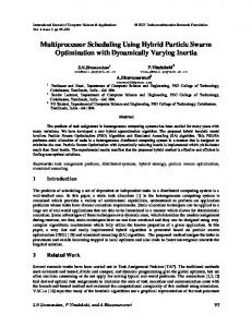
Our theoretical results can be applied in many real-world applications, such as the power management problem of a multiple-speed disk [7] and the dynamic voltage scheduling (DVS) problem of a variable speed processor [5]. In this section, we use a DVS example to illustrate the effectiveness of our result.

Mode Voltage (v) Speed (Kbps) Power (w)

1

Nomalized Total Energy

The optimal P¯ can be obtained by minimizing (11) with respect to (σ1 , σ2 ). Hence,  (ri − r0 )pj + (r0 − rj )pi (σ1 , σ2 ) = arg min ri − rj (i,j)∈I×J s ! pm ks (ri − r0 )(r0 − rj ) . (12) +2 ri − rj

4 2.5 8333 1.16

5 3.3 11000 2.01

The power of a processor is approximately proportional to the square of its supply voltage; and DVS tries to reduce the system power consumption by appropriately arranging the supply voltages for a given task [6]. In our simulation, the interacting components X and Y are a processor and a video, respectively. Suppose that the video consists of 45000 frames; each is of size 300Kb. As a strict requirement, the video data must be processed by X at a constant speed 25 frame/sec, or equivalently, 7500Kb/sec. We assume that the processor has five power modes and the voltage, speed, and power in each mode are given in Table I. In addition, we suppose that the power parameter of the buffer is pm = 8.24 ∗ 10−8 W/B and the switching cost ks varies from 1mJ to 100mJ. One way to reduce the power consumption is to use the highest speed to finish a frame and turn off the processor for the rest of the frame period. We refer this method as Scheme 1, while Scheme 2 represents the proposed method which schedules the voltages according to the formulas in Theorem 1. In Figure 6, for each scheme we plot the corresponding energy consumption of processing the whole video as a function of the switching costs. The result is normalized with respect to the energy cost of Scheme 1 for each switching cost. It is clear that the proposed method can save at least 30% of energy compared with the heuristic method and more energy can be saved as the switching cost increases. In practice, the switching cost is application dependent [5]. The proposed method can guarantee a minimum energy consumption for any switching cost. V. C ONCLUSION This paper studies the optimal power management problem of two interacting components with a buffer. We assume that the component to be controlled has multiple power

0

−2

−1

10

10

Switching Cost K (J) s

Fig. 6.

Simulation Result

modes and model the overall system as a hybrid system. The power management problem is formulated as an optimal control problem and the optimal buffer size and the optimal switching strategy are derived analytically. Future research will focus on the case where the data consumption rate r0 is time varying or random. R EFERENCES [1] L. Benini and G. D. Micheli. System level power optimization: Techiniques and tools. ACM Transactions on Design and Automation of Electronic Systems, 5(2):115–192, April 2000. [2] L. Cai and Y.-H. Lu. Energy management using buffer memory for streaming data. IEEE Transactions on Computer-Aided Design of Integrated Circuits and Systems, pages 141–152, February 2005. [3] J. Hu and Y.-H. Lu. Buffer management for power reduction using hybrid control. In Proc. IEEE Int. Conf. Decision and Control, pages 6997–7002, Seville, Spain, 2005. [4] J. Ridenour, J. Hu, and Y.-H. Lu. Low power buffer management using hybrid control. In Proc. American Control Conference, 2006. [5] T. D. Burd and R. W. Brodersen. Design issues for dynamic voltage scaling. In Proceedings of the international symposium on Low power electronics and design, pages 9–14. ACM Press, 2000. [6] T. Ishihara and H. Yasuura. Voltage scheduling problem for dynamically variable voltage processors. In Proceedings of the international symposium on Low power electronics and design, pages 197 – 202. ACM Press, 1998. [7] S. Gurumurthi, A. Sivasubramaniam, M. Kandemir, and H. Franke. Drpm: Dynamic speed control for power management in server class disks. In Proceedings of the International Symposium on Computer Architecture (ISCA), pages 169–179, June 2003. [8] R. Alur, T. Henzinger, G. Lafferriere, and G. J. Pappas. Discrete abstractions of hybrid systems. Proceedings of the IEEE, 88(2):971– 984, 2000. [9] S. Hedlund and A. Rantzer. Optimal control of hybrid system. In Proceedings of the IEEE Conference on Decision and Control, volume 4, pages 3972–3977, Phoenix, AZ, December 1999. [10] M. Egerstedt, Y. Wardi, and F. Delmotte. Optimal control of switching times in switched dynamical systems. IEEE Transactions on Automatic Control, 51(1):110–115, 2006. [11] X. Xu and P.J. Antsaklis. Optimal control of switched systems based on parameterization of the switching instants. IEEE Transactions on Automatic Control, 49(1):2–16, 2004. [12] S. C. Bengea and R. A. DeCarlo. Optimal control of switching systems. Automatica, 41(1):11–27, 2005. [13] Y.-H. Lu, L. Benini, and G. D. Micheli. Dynamic frequency scaling with buffer insertion for mixed workloads. IEEE Transactions on Computer-Aided Design of Integrated Circuits and Systems, pages 1284–1305, November 2002.