This paper describes a framework for student modeling in Intelligent Tutoring Systems that ... the information in the Ba
On-Line Student Modeling for Coached Problem Solving Using Bayesian Networks �
Cristina Conati , Abigail S. Gertner , Kurt VanLehn
�� �
, and Marek J. Druzdzel
�� ���
�
�
Intelligent Systems Program, University of Pittsburgh, PA, U.S.A. Learning Research and Development Center, University of Pittsburgh, PA, U.S.A. � Department of Information Science, University of Pittsburgh, PA, U.S.A.
Abstract. This paper describes the student modeling component of A NDES, an Intelligent Tutoring System for Newtonian physics. A NDES’ student model uses a Bayesian network to do long-term knowledge assessment, plan recognition and prediction of students’ actions during problem solving. The network is updated in real time, using an approximate anytime algorithm based on stochastic sampling, as a student solves problems with A NDES. The information in the student model is used by A NDES’ Help system to tailor its support when the student reaches impasses in the problem solving process. In this paper, we describe the knowledge structures represented in the student model and discuss the implementation of the Bayesian network assessor. We also present a preliminary evaluation of the time performance of stochastic sampling algorithms to update the network.
To appear in Proceedings of the Sixth International Conference on User Modeling (UM-97), Sardinia, Italy. June 1997.
1 Introduction A NDES is an Intelligent Tutoring System that teaches Newtonian physics via coached problem solving (VanLehn, 1996), a method of teaching cognitive skills in which the tutor and the student collaborate to solve problems. In coached problem solving, the initiative in the student-tutor interaction changes according to the progress being made. As long as the student proceeds along a correct solution, the tutor merely indicates agreement with each step. When the student stumbles on a certain part of the problem, the tutor helps the student overcome the impasse by providing tailored hints that lead the student back to the correct solution path. In this setting, the critical problem for the tutor is to interpret the student’s actions and the line of reasoning that the student is following. To perform this task the tutor needs a student model that performs plan recognition (Charniak and Goldman, 1993; Genesereth, 1982; Huber et al., 1994; Pynadath and Wellman, 1995).
This research is supported by AFOSR under grant number F49620-96-1-0180, by ONR’s Cognitive Science Division under grant N00014-96-1-0260 and by DARPA’s Computer Aided Education and Training Initiative under grant N66001-95-C-8367. In addition, Dr. Druzdzel was supported by the National Science Foundation under Faculty Early Career Development (CAREER) Program, grant IRI–9624629. We would like to thank Zhendong Niu and Yan Lin for programming support.
Inferring an agent’s plan from a partial sequence of observable actions is a task that involves inherent uncertainty since often the same observable actions can belong to different plans. In coached problem solving, two additional sources of uncertainty increase the difficulty of the plan recognition task. Firstly, coached problem solving often involves interactions in which most of the important reasoning is hidden from the coach’s view. This is especially true when the coach decides to reduce the level of guidance in the problem solving process by no longer requiring the student to explicitly show the problem solving steps that can be performed mentally. Secondly, there is additional uncertainty regarding the student’s level of understanding of the domain theory and, therefore, the kind of knowledge that she can bring to bear in generating solution plans. This paper describes a framework for student modeling in Intelligent Tutoring Systems that takes into account both the uncertainty about the student’s plans and the uncertainty about her knowledge state. The framework uses a Bayesian network (Pearl, 1988) to represent and update the student model on-line, during problem solving. The student model is constructed by the Assessor module of A NDES and it is used to tailor A NDES’ coaching to the problem solving performance of each individual student.
2 The A NDES Student Modeling Framework A NDES’ student model represents a significant contribution to research in probabilistic user modeling for three reasons. First, the model uses a probabilistic framework to perform three kinds of assessment: (1) plan recognition, inferring the most likely strategy among possible alternatives the student is following, (2) prediction of students’ goals and actions, and (3) long-term assessment of the student’s domain knowledge. None of the existing systems that perform probabilistic user modeling seem to combine all three of these functions (Jameson, 1996). A NDES’ Assessor evolves from POLA (Conati and VanLehn, 1996a, 1996b), our first attempt at a student model for coached problem solving. Unlike POLA, which exploited only the diagnostic capabilities of its Bayesian network, the Assessor also provides predictions about the inferences that the student may have made but not yet expressed via actual solution steps, and the inferences that may cause problems. These predictions will provide A NDES with more principled information to generate effective coached problem solving than the heuristics used by POLA. Second, this model performs plan recognition by integrating in a principled way knowledge about the student’s behavior and mental state with knowledge about the available plans. While substantial research has been devoted to using probabilistic reasoning frameworks to deal with the inherent uncertainty of the plan recognition task (Carberry, 1990; Charniak and Goldman, 1993; Huber et al., 1994; Pynadath and Wellman, 1995), none of it encompasses applications where much uncertainty concerns the knowledge that the user has to generate the plans. If the assumption that the planning agent has complete and correct knowledge is reasonable in many plan recognition applications, it is certainly not realistic for plan recognition in an Intelligent Tutoring System, whose primary goal is to improve the incorrect and incomplete knowledge of the student. Nonetheless, the few existing systems that perform plan recognition for intelligent tutoring systems rely on a library of available plans, without taking into consideration the student’s degree of mastery in the target domain (Genesereth, 1982; Kohen and Greer, 1993; Ross and Lewis, 1988). The model-tracing tutors of Anderson et al. (1995) assess both a
student’s mastery of the domain and the solution that the student is following during problem solving, but they do not integrate the two kinds of assessment. They apply probabilistic methods only for knowledge assessment and reduce the complexity of plan recognition by restricting the number of acceptable solutions the student can follow and by asking the student when there is still some ambiguity. Third, the student model will be used in real-time to tailor the coaching of students’ problem solving. Bayesian networks have been used for the off-line assessment of student’s domain knowledge from problem solving performance (Collins et al., 1996; Gitomer et al., 1995; Martin and VanLehn, 1995; Mislevy, 1995; Petrushin and Sinitsa, 1993), but none of these systems uses the information in the Bayesian student model to guide a real-time tutorial dialogue. One reason for this may be that belief updating in Bayesian networks is in the worst case NP-Hard, and this intractability often manifests itself when the application calls for large and complex models, as is the case with Intelligent Tutoring Systems. In A NDES, the computational complexity of the network evaluation is definitely an issue. Our networks are fine-grained models of the complex reasoning involved in physics problem solving and can contain from 200 nodes for a simple problem to 1000 nodes for a complex one. Moreover, since A NDES will be part of the curriculum of the introductory physics course at the United States Naval Academy, its response time will be a decisive factor for the success of the innovation that A NDES represents for the classical curriculum. We are devoting great effort to obtain acceptable performances from our student model by using approximate anytime algorithms based on stochastic sampling.
3 The A NDES Tutoring System The A NDES project is a joint collaboration between the University of Pittsburgh and the Naval Academy involving about 10 researchers and programmers. Beginning in 1998, A NDES will be used by approximately 200 students per semester in the introductory physics class at the United States Naval Academy. A NDES is implemented in Allegro Common Lisp and Microsoft Visual C++ on a Pentium PC running Windows 95. A NDES has a modular architecture comprising, besides the Assessor, a graphical Workbench with which the student solves physics problems, an Action Interpreter that provides immediate feedback to student actions, and a Help System.1 A NDES’ Help System comprises three separate modules responsible for Procedural, Conceptual, and Meta Help (VanLehn, 1996). The probabilities calculated by the Assessor will be used by the Help modules, both to diagnose which concepts the student needs more detailed tutoring on, and to predict what hints are most relevant to the student’s current strategy. The knowledge assessment capabilities of the Assessor can be used to select appropriate problems for the student, and can also serve as an additional assessment tool for the teacher. 1
All modules except the Help System have already been implemented. The Help System will be implemented in the next version of A NDES.
4 Probabilistic Assessment in A NDES 4.1 The Solution Graph Representation One of the issues that must be considered when using Bayesian networks for plan recognition is where the network and its parameters come from. Designing the network by hand for each plan recognition task requires a considerable knowledge engineering effort and it is an unacceptable option in a system like A NDES, where teachers should be able to easily extend and modify the set of physics problems available to students. In POLA we solved this problem by adopting the approach, introduced by Huber et al. (1994) and Martin and VanLehn (1995), of automatically constructing its Bayesian networks from the output of a problem solver that generated all the acceptable solutions and solution plans to a problem. Similarly, the solution graph structure used by A NDES’ Assessor is generated prior to run time by a rule-based physics problem solver. The rules are being developed in collaboration with three physics professors from the Naval Academy, who are the domain experts for the A NDES project. Since the output of the problem solver will be used to model the student’s activity and make tutoring decisions, it is important to choose an appropriate grain size for its knowledge representation. We have based A NDES’ problem-solving rules on the representation used by Cascade (VanLehn et al., 1992), a computational model of knowledge acquisition developed from an analysis of protocols of students studying worked example problems. This analysis results in a rather fine grain size which, as we will discuss in Section 4.4, can produce large models that pose a real challenge for current Bayesian network updating algorithms. However, we argue that such a fine-grained representation is necessary for making the kinds of tutoring decisions A NDES will make. Both POLA’s and A NDES’ problem solvers contain knowledge about the qualitative and quantitative reasoning necessary to solve complex physics problems. However, while POLA’s problem solver generates plain sequences of solution steps (Conati and VanLehn, 1996a), A N DES’ problem solver has explicit knowledge about the abstract planning steps that an expert might use to solve problems, and about which A NDES will tutor students. Thus, it produces a hierarchical dependency network including, in addition to all acceptable solutions to the problem in terms of qualitative propositions and equations, the abstract plans for how to generate those solutions. This network is called the problem solution graph, and is the starting point for the construction of the Assessor module’s Bayesian network. The Problem Solver starts with a set of propositions describing the situation, and a goal statement that identifies the sought quantity for the problem. It begins by iteratively applying rules from its rule set, generating sub-goals and intermediate propositions. When it reaches an equation, it determines what quantities in the equation are still unknown and forms new sub-goals to find the values of those quantities, so that it will be possible to solve for the sought quantity when all the sub-goals have been achieved. For example, consider the problem statement shown in Figure 1A. The problem solver starts
�� . From this, it forms the with the top-level goal of finding the value of the normal force sub-goal of using Newton’s second law to find this value. Next, it generates three sub-goals corresponding to the three high level steps specified in the procedure to apply Newton’s second law ( ��������������� � ): (1) choose a body/bodies to which to apply the law, (2) identify all the
*+.0/0, #'60,� !�" # /�.01(# 4 $+*',5/�.(1(# 2�.0$3"(/�.(1(# !�" #%$'&(&�" ) *+$-, ) .0/ /�.(1(# 7 , $-, #'2389/�.(1(# |
Z
= > ? @A= B > CED ?
Z\[�] ^`_0acb ZedH^Jf�gih5jNjPkJlnmporq+s5j-tEjX^�u t ^�vc^JfwhLt h([x] s�y0Zruz^�t {zs3qH[�] ^`_0acb |}d%^Jf gTh5j3j9~(lnmponq-s�j-t jP^Juet ^Jv^`f[�] ^�_0apZTy {zh0tz j%t {zsLux^`qEgTh(]xf'^�q-_5ss0xs(qEt s�
r[` t {xsAt h0[�] sr^�ue[x] ^`_0apZ O
'* :�.(.(7;# *+.0FA&�.0!(/�1 < .(1+8
1(# 4 ) /�# < .(1() #+7 K *+.0FA&�.0!(/�1�W OXS%Y M ��� S
4 ) /�1 = > ? *':�.(.(7;# < .(1+8
< .(1+89*+:�.() *3# 7 , $', #+238 *':�.(.(7;# < .(1() #+7 1(# 4 ) /�# < .(1+8
, 8 = #'GH, .0/JI 7 4 .0 4 .0 *+#
, 8 = '# GH, .0/JI 7 " $;GLK = > ? M
GP ) , # *+.0FA&�.0/�#'/0, #+Q0!�$-, ) .0/�7
*':�.(.(7-# 7E#+&�$+ $-, # < .(1() #+7 ) 1(#'/0, ) 4 89$+" " 4 .0 *+#37 (1 # 4 ) /�# < .(1() #+7;K OPR S M
ST) 7U$ < .(1+8
OV) 7U$ < .(1+8
GP ) , # *+.0FA&�.0/�#'/0, #3QN/�7 4 ) /�1 4 .N *'#N7 .0/PO
���
���
Figure 1. A physics problem and corresponding solution graph segment.
forces on the body, (3) write the component equations for ���(� � ������ . The resulting plan is a partially ordered network of goals and sub-goals leading from the top-level goal to a set of equations that are sufficient to solve for the sought quantity. Figure 1B shows a section of the solution graph for the problem in Figure 1A involving the application of Newton’s second law to find the value of the normal force. In the following section we use this example to show how the solution graph is converted into a Bayesian network by the Assessor module, and describe the different types of nodes in the network and the relationships between them. 4.2 The Assessor’s Bayesian Network The Assessor Bayesian network consists of two parts, one static and one dynamic. The static part is built when the A NDES domain knowledge is defined and is maintained across problems. The dynamic part is automatically generated when the student selects a new problem and is discarded when the problem is solved. The following sections will describe the semantics and the structure of the nodes in the static and in the dynamic network. As far as the parameterization of the network is concerned, we mainly rely on canonical interactions, known as Noisy/Leaky-OR and Noisy/Leaky-AND (Henrion, 1989), to automatically specify the conditional probabilities in the network. These canonical interactions are good approximations of the probabilistic relationships in the network and provide a fundamental advantage: they reduce logarithmically the number of conditional probabilities required to specify the interaction between a node and its parents by requiring only a single parameter that represents the noise or the leak in the canonical interaction. At the moment the parameters in the canonical interactions, along with the prior probabilities in the network, derive from our rough estimates. We plan to refine them based on the judgment of the domain experts in the A NDES project.
The static part of the Assessor. The static part of the Assessor consists of Rule nodes and Context-Rule nodes. We use these two kinds of nodes to model what it means for a student to know a piece of physics knowledge. Our definition is that a student knows a rule when she is able to apply it correctly whenever it is required to solve a problem, i.e. in all possible contexts. In POLA, the student’s knowledge of a rule formalizing a piece of physics knowledge was represented by the probability of a Rule node that increased by the same amount every time the student performed an action that entailed the correct application of the rule, independent of the context of the application. However, for many physics rules there are categories of problems (contexts) that entail different levels of difficulty in applying the rule. For example, it is easier to identify correctly the direction of the normal force acting on the body in the problem in Figure 1A than in a problem in which the body slides on an inclined plane. Thus, the correct application of the rule to problems in different categories provide different evidence that the student knows the rule. In A NDES, Rule and Context-Rule nodes have been introduced to model this relationship between knowledge and application. Rule nodes in the static part of the Assessor represent generic physics rules. They have binary values T and F, where �(\e'�\� is the probability that the student can apply the rule in every situation. The prior probabilities of Rule nodes are given with the solution graph for the problem. At the moment, all the Rule nodes are initialized with a probability of eE , but we plan to obtain more realistic values from an analysis of students’ performance on a diagnostic pre-test that is administered at the Naval Academy at the beginning of the introductory physics course. Context-Rule nodes represent the application of physics knowledge in specific problem solving contexts. Each Context-Rule corresponds to a production rule in A NDES’ problem solver. Context-Rules are shown in Figure 1B as the octagonal nodes. For each Rule node the Assessor contains as many Context-Rule nodes as there are contexts defined for that rule. Context-Rule nodes have binary values T and F, where � Context-Rule �\� is the probability that the student knows how to apply the rule to every problem in the corresponding context. Each Context-Rule node has only one parent, the Rule node representing the corresponding rule. � Context-Rule� e+�\� is always equal to 1, since by definition ��e+�\� means that the student can apply the rule in any context. � Context-Rule� e+�� represents the probability that the student can apply the general rule in the corresponding context even if she cannot apply it in all contexts. This probability implicitly defines the level of difficulty of a context for the application of a rule—the easier the context, the higher this conditional probability. As we will illustrate in Section 4.3, the marginal probabilities of Rules and Context-Rules will carry over from one problem to the next, encoding the long-term knowledge assessment for each student that has been solving problems with Andes. The structure of the static part of the student model entails two independence assumptions. The first assumption is that Rule nodes are independent of each other, the second is that ContextRule nodes are conditionally independent given Rule nodes. These assumptions simplify the modeling task and reduce the computational complexity of belief updating. However, they do not always hold in the physics domain, and we are planning to work with the domain experts to model correctly the existing dependencies. The dynamic part of the Assessor. The dynamic part of the Assessor contains Context-Rule nodes and four additional types of nodes: Fact, Goal, Rule-Application and Strategy nodes. All
the nodes are read into the network from the solution graph for the current problem at the beginning of problem solving. The structure of the solution graph already encodes the causal structure of the problem solutions and therefore is maintained in the Bayesian network. For example, a segment of the Bayesian network created for the problem in Figure 1A corresponds exactly to the solution graph segment in Figure 1B. Fact and Goal nodes. Fact and Goal nodes look the same from the point of view of the Bayesian network. They both represent information that is derived while solving a problem by applying rules from the knowledge base. The difference between Goal and Fact nodes is in their meaning to the help system: The probability of Goal nodes will be used to construct hints focused on the qualitative analysis of the problem and on the planning of the solution, while the probabilities of Fact nodes will be used to provide more specific hints on the actual solution steps. Goal and Fact nodes have binary values T and F. �(A �\� is the probability that the student knows that fact. ��¡¢9L�\� is the probability that the student has been pursuing that goal. A weakness of the current representation of Goal nodes is that the probability �5¡¢}A�\� does not specify whether the student has simply established the goal during the problem solving process or she has also accomplished it. The distinction between established and accomplished goals is crucial for the help system since the student may need help in reaching a goal that she has established but not on a goal that she has already accomplished. At the moment we use a separate procedure to detect the goals that have already been accomplished when the Help System needs to intervene. Goal and Fact nodes have as many parents as there are ways to derive them. The conditional probabilities between Fact and Goal nodes and their parents are described by a Leaky-OR relationship (Pearl, 1988). This models the fact that a Fact or Goal node is true if the student performed at least one of the inferences that derive it, but it can also be true when none of these inferences happened because the student may use an alternative way to generate the result, such as guessing or drawing an analogy to another problem’s solution. Strategy nodes. Strategy nodes represent points where the student can choose among alternative plans to solve a problem. Strategy nodes are the only non-binary nodes in the network: they have as many values as there are alternative strategies. The children of Strategy nodes are the RuleApplication nodes that represent the implementation of the different strategies. In Figure 1B, for example, the strategy node body choice strategy points to the two application nodes representing respectively the decisions to choose block A and block B as separate bodies and to choose as a body the compound of the two blocks. The values of a Strategy node are mutually exclusive strategies which represent the fact that, at each solution step, the student is following exactly one of the represented strategies. Thus, evidence for one strategy decreases the probability of the others. Like Rule nodes, strategy nodes have no parents in the solution graph. Rule-Application nodes. Rule-Application nodes connect Context-Rule, Strategy, Fact and Goal nodes to new derived Fact and Goal nodes. Rule-Application nodes have values T and F. � Rule-Application �\� represents the probability that the student has applied the corresponding Context-Rule to the facts and goals representing its preconditions to derive the facts and goals representing its conclusions.
ÉNÊwÊ É0ËwÌ
±'°(· ©z»¼±N¦H´p½+¨ ¾ ¯x»\¿'· ¹-º À z¤ ¥}¦§¦L¨�© ¨J©x®9¯z°�¯x±N© ª ¦§«P¬+©¨
¤z¥}¦§¦L¨J© ª ¦§«P¬+©¨
«§© ¶ ¬E´}© ª ¦§«P¬+©¨ ¿0¤%¦H²\®9¦H³§´}«9ÆEÁÇøÈNÀ É5ÐwÐ £E£E£
É0ËwÌ
±'°0· ©U»¼±N¦H´p½'¨ ¶ ¦H° ¶ ¦H°�¤�©
É0ËwÌ
¤z¥}¦§¦L¨J© ª ¦§«H
ÉNËÏÌTÓzÉ0ËwÌ ª ¦§«H¤z¥}¦P¬'¤© ¨�±+°5¯U±3©�µX
ÉNËÏÌ ¤z¥}¦§¦L¨�© ¤%¦H²\®9¦H³§´}« ª ¦§«H
¶ ¬;´}«¸· ¹-º
É3ÎÏÑ «§© ¶ ¬ ´}© ª ¦§«H
É�ÐTÒ ÃĬ3¨Å¯ ª ¦§«H
«§© ¶ ¬E´}© ª ¦§«P¬'©%¨J¿NÁ  ÃwÀ
É3ÍÏÎ
É0ËwÌ ¬+«§©x´§±3¬ ¶ ¶ ¦H°J¤�©¨
ÉNËwÌ É5ÐwÐ É�ÐÅÎ ¶ ¬;´}« ¶ ¦H°�¤�©%¨ ¦H´Á
É5ÐiË Á¬3¨T¯ ª ¦§«H
£E£E£
Figure 2. The network before observing A-is-a-body.
The parents of each Rule-Application node include exactly one Context-Rule, some number of Fact and/or Goal nodes, and optionally one Strategy node. The probabilistic relationship between the Rule-Application node and its parents is a Noisy-AND. The noise in the AND relationship models the probability that the student will not apply the rule even if all the preconditions are known. 4.3 Example of Propagation of Evidence in the Assessor Suppose that a student is trying to solve the problem in Figure 1A and that her first action is to select Block A as the body. In response to this action the fact node A-is-a-body is clamped to T. Figure 2 shows the probabilities in the network before the action. Note that the a priori probability of Fact and Goal nodes is rather low, especially when the evidence is far from the givens in the network, because of the large number of inferences which must be made in conjunction in order to derive the corresponding facts and goals. After the first action, evidence propagates upward increasing the probability of its parent nodes define-body and define-bodies-(A,B), as shown in Figure 3. The upward propagation also increases slightly the probability of the value separate-bodies of the Strategy node body-choicestrategy, represented in Figure 3 by the right number of the pair associated to the strategy node. The changes in the probabilities of nodes that are ancestors of the observed action represent the model’s assessment of what knowledge the student has brought to bear to generate the action. The fact that such changes are quite modest is due to the leak in the Leaky-OR relation between the observed Fact node and its parent Application node. Given the current low probability of the Application node the leak absorbs most of the evidence provided by the student’s action.
ôNõwõ ô0öúù
ÕzÖ}ק×LØJÙ Ú ×§ÛPÜ+ÙØ ô0ü�õ
Û Ù æ ÜEä}Ù Ú ×§ÛPÜ+ÙØ § í(Õ×Hâ\Þ9×Hã§ä}Û9ò;ïÇñó î ô5ùwù ÔEÔEÔ
á'à0Ýç ÙUê¼áN×Häpë'Ø æ ×Hà æ ×Hà�Õ�Ù
ô0öw÷
ÕzÖ}ק×LØJÙ Ú § × ÛHÝ á'à(Ýç Ùzê¼áN×Häpë+Ø ì ßxê\í'ç è-é î
3ô þÏõiÿzô0öúù Ú ×§ÛHÝÕzÖ}×PÜ'ÕÙ Ø�á+à5ßUá3Ù�åXÝ
ôNöÏ÷ ÕzÖ}ק×LØ�Ù Õ%×Hâ\Þ9×Hã§ä}Û Ú ×§ÛHÝ
æ Ü;ä}Û¸ç è-é
zÕ Ö}ק×LØ�Ù ØJÙxÞ9ßzà�ßxáNÙ Ú ×§ÛPÜ+ÙØ ô3ûö
Û§Ù æ Ü ä}Ù Ú ×§ÛHÝ
ôNûÏý ñÄÜ3ØÅß Ú ×§ÛHÝ
ô3øwø
ôNöúù
ô3ûwû Û Ù æ ÜEä}Ù § Ú ×§ÛPÜ'Ù%ØJíNï ð ñ î
ùiô0÷w÷ ïÜ3ØTß Ú ×§ÛHÝ
ô0öw÷ Ü+Û§Ùxä§á3Ü æ Ý æ ×HàJÕ�ÙØ
æ Ü;ä}Û æ ×Hà�Õ�Ù%ôNØ ûwþ ×Häï ÔEÔEÔ
Figure 3. The network after observing A-is-a-body.
In general the influence of the leaks in the network will decrease as the student performs more correct actions. At this point, downward propagation changes the probabilities of yet to be observed nodes, thus predicting what inferences the student is likely to make. In particular, the relationship enforced by the Strategy node body-choice-strategy on its children will slightly diminish the probability of the Goal node define-bodies(AB). Moreover, the increased probability of the Goal node define-bodies(A,B) will propagate downward to increase the probability of the Fact node B-isa-body while the increased probability of the Fact node A-is-a-body will slightly increase the probability of the Goal node find-Forces-on(A), as shown in Figure 3. If the student asks for help after having selected block A as a body, the Help System separates the nodes that are ancestors of the performed actions from the nodes that can be directly or indirectly derived from the performed actions. The Goal and Fact nodes in the latter group represent the set of inferences that the student has not yet expressed as actions, and from which the Help System can choose to suggest to the student how to proceed. The probabilities of these nodes will aid the Help System in deciding what particular inference to choose. Once the student has completed a problem, the dynamic part of the Bayesian network is eliminated and the probabilities assessed for the Context-Rules that were included in the solution graph for the problem are propagated in the static part of the network. Upward propagation in the static network will modify the probability of Rule nodes, generating long-term assessment of the student physics knowledge. Downward propagation from Rule nodes to Context-Rule nodes not involved in the last solved problem generates predictions of how easy it will be for the student to apply the corresponding rules in different contexts.
Table 1. Performance of Likelihood Sampling algorithm.
Precision
������ ���� � ���� �
Number of samples
Run time (seconds)
1,374,000 362,000 5,000
400 140 30
4.4 Analysis of the Update Algorithms’ Performance The use of approximate algorithms was a forced choice for the belief update of the Assessor, since exact algorithms run out of memory on most of our networks and have unacceptable performance on the others. However, they also naturally fit the task because, as they are anytime algorithms, they produce approximate results rather quickly and the longer they run the more precise results they provide. As we described in previous sections, A NDES’ Assessor is updated every time the student performs a new action, but its assessment is needed only when the student asks for help. The Bayesian network is updated in a background thread, so the student can go on working on the Workbench without any awareness that the network calculation is happening, until she invokes the Help System. Only then the student may have to wait until the results of the belief updating algorithm are precise enough for the Help system to generate a reliable response. We have tested the time taken by two different stochastic sampling algorithms, Logic Sampling and Likelihood Sampling (Cousins et al., 1993), to bring the probability of every node in a representative network within a small threshold precision. The network we tested had to be small enough to also run an exact evaluation algorithm to produce the exact posterior probabilities for comparison. The network was generated from a very simple problem and had 110 nodes. Stochastic sampling algorithms typically do not perform well on networks with unlikely evidence, as our networks often are, and we found that the Likelihood Sampling algorithm was the only one with acceptable performances on our test network. Table 1 shows the number of samples and running time it took Likelihood Sampling to get all nodes in the network within a precision of p� , e , and e � , compared with the probabilities calculated by the exact algorithm, when all actions that form the problem solutions have been observed. The running time of stochastic algorithms increases approximately linearly with the number of nodes. Therefore, given the results in Table 1, Likelihood Sampling would take several minutes to update to high precision our largest networks, which are up to ten times larger than our test network. On the other hand, we have observed that the students who have used A NDES so far usually pause for a while before asking for help and the Assessor has some time to run the updating algorithm. Besides, when Likelihood Sampling reaches the p precision for all the nodes 98% of the nodes are already within e� precision, and when it reaches the e � precision 98% of the nodes are already within e and 66% of the nodes are within p� precision. Therefore, it may be the case that we won’t need dramatically better updating time in order for the Assessor to reach acceptable performances. While we intend to continue to work on improving the speed of
the Assessor’s belief updating, we also plan to run pilot subjects to measure the average waiting time before a help request, and to evaluate what precision thresholds will allow for adequate assessment.
5 Conclusions and Future Work The Bayesian student modeling framework presented in this paper contributes to research on probabilistic user modeling in a number of ways. First, it uses a probabilistic framework to perform three kinds of assessment: plan recognition, prediction of students’ goals and actions, and long-term assessment of the student’s domain knowledge. Second, it performs plan recognition by integrating in a principled way knowledge about the student’s behavior and mental state with knowledge about the available plans. Third, it represents a substantial effort toward obtaining acceptable real time performance in the evaluation of very complex Bayesian networks (ranging from 200 to 1000 nodes) to be used for the on-line tailoring of the dialogue with the student. In this paper we have described in detail the structure of the Bayesian network and how it is automatically constructed from the output of a problem solver that generates all of the acceptable abstract solution plans and actions sequences to solve a problem. We have also presented a preliminary evaluation of the performance of the Assessor’s update algorithms on a representative network. A number of issues remain to be addressed for the A NDES Assessor. The first is to improve the performance of belief updating. We are currently exploring the possibility of applying methods based on relevance and focused reasoning (Druzdzel and Suermondt, 1994; Lin and Druzdzel, 1997), which we believe will lead to a significant speedup of our algorithms. Second, the knowledge base used by the problem solver will be further developed. In particular, we plan to add incorrect rules corresponding to common physics misconceptions. Third, we will work with our domain experts to refine the parameters in the Bayesian networks and to model dependencies among physics rules. Fourth, we will explore how to make the Assessor able to take into account student actions that do not correspond to a correct entry in the solution graph, such as erroneous entries and deletion of previous entries. More issues could be addressed to refine the accuracy of the student model, such as how to explicitly represent time in the Bayesian network to take into consideration the temporal sequencing of the student actions and changes in the students’ knowledge due to forgetting. On the other hand, as Self (1988) points out, the complexity of a student model should always be calibrated against the accuracy of its predictions. We believe that it is important to continuously verify the adequacy of the model as we develop it, through formative evaluations with the intended users of the system. A NDES’ Assessor will be incrementally modified and improved as we gain insight from these evaluations.
References Anderson, J., Corbett, A., Koedinger, K., and Pelletier, R. (1995). Cognitive tutors: Lessons learned. The Journal of the Learning Sciences 4(2):167–207. Carberry, S. (1990). Incorporating default inferences into plan recognition. In Proceedings of the 8th National Conference on Artificial Intelligence, 471–478.
Charniak, E., and Goldman, R. (1993). A Bayesian model of plan recognition. Artificial Intelligence 64(1):53–79. Collins, J. A., Greer, J. E., and Huang, S. X. (1996). Adaptive assessment using granularity hierarchies and Bayesian nets. In Frasson, C., Gauthier, G., and Lesgold, A., eds., Proceedings of the 3rd International Conference on Intelligent Tutoring Systems ITS ’96. Berlin: Springer. 569–577. Conati, C., and VanLehn, K. (1996a). POLA: a student modeling framework for Probabilistic On-Line Assessment of problem solving performance. In Proceedings of the 5th International Conference on User Modeling, 75–82. Conati, C., and VanLehn, K. (1996b). Probabilistic plan recognition for cognitive apprenticeship. In Proceedings of the 18th Annual Conference of the Cognitive Science Society, 403–408. Cousins, S., Chen, W., and Frisse, M. (1993). A tutorial introduction to stochastic simulation algorithms for belief networks. Artificial Intelligence in Medicine 5:315–340. Druzdzel, M. J., and Suermondt, H. J. (1994). Relevance in probabilistic models: “Backyards” in a “small world”. In Working notes of the AAAI-1994 Fall Symposium Series: Relevance, 60–63. Genesereth, M. (1982). The role of plans in intelligent teaching systems. In Sleeman, D., and Brown, J. S., eds., Intelligent Tutoring Systems. New York: Academic Press. 137–156. Gitomer, D., Steinberg, H., S., L., and Mislevy, R. J. (1995). Diagnostic assessment of troubleshooting skill in an intelligent tutoring system. In Nichols, P., Chipman, S., and Brennan, R., L., eds., Cognitively Diagnostic Assessment. Hillsdale, NJ: Erlbaum. Henrion, M. (1989). Some practical issues in constructing belief networks. In Kanal, L. N., Levitt, T. S., and Lemmer, J. F., eds., Proceedings of the 3rd Conference on Uncertainty in Artificial Intelligence, 161–173. Elsevier Science Publishers. Huber, M., Durfee, E., and Wellman, M. (1994). The automated mapping of plans for plan recognition. In Proceedings of the 10th Conference on Uncertainty in Artificial Intelligence, 344–351. Jameson, A. (1996). Numerical uncertainty management in user and student modeling: An overview of systems and issues. User Modeling and User-Adapted Interaction 5(3-4):193–251. Kohen, G., and Greer, J. (1993). Recognizing plans in instructional systems using granularity. In Proceedings of the 4th International Conference on User Modeling, 133–138. Lin, Y., and Druzdzel, M. J. (1997). Computational advantages of relevance reasoning in Bayesian belief networks. In Proceedings of the 13th Conference on Uncertainty in Artificial Intelligence. to appear. Martin, J., and VanLehn, K. (1995). A Bayesian approach to cognitive assessment. In Nichols, P., Chipman, S., and Brennan, R. L., eds., Cognitively Diagnostic Assessment. Hillsdale, NJ: Erlbaum. Mislevy, R. J. (1995). Probability-based inference in cognitive diagnosis. In Nichols, P., Chipman, S., and Brennan, R., L., eds., Cognitively Diagnostic Assessment. Hillsdale, NJ: Erlbaum. Pearl, J. (1988). Probabilistic Reasoning in Intelligent Systems: Networks of Plausible inference. Los Altos, CA: Morgan Kaufmann. Petrushin, V. A., and Sinitsa, K. M. (1993). Using probabilistic reasoning techniques for learner modeling. In Proceedings of the 1993 World Conference on AI and Education, 426–432. Pynadath, D. V., and Wellman, M. P. (1995). Accounting for context in plan recognition, with application to traffic monitoring. In Proceedings of the 11h Conference on Uncertainty in Artificial Intelligence, 472–481. Ross, P., and Lewis, J. (1988). Plan recognition for intelligent tutoring systems. In Ercoli, P., and Lewis, R., eds., Artificial Intelligence Tools in Education. Amsterdam: Elsevier Science Publishers. 29–37. Self, J. (1988). Bypassing the intractable problem of student modeling. In Proceedings of Intelligent Tutoring Systems ’88, 18–24. VanLehn, K., Jones, R. M., and Chi, M. T. H. (1992). A model of the self-explanation effect. The Journal of the Learning Sciences 2(1):1–59. VanLehn, K. (1996). Conceptual and meta learning during coached problem solving. In Frasson, C., Gauthier, G., and Lesgold, A., eds., Proceedings of the 3rd International Conference on Intelligent Tutoring Systems ITS ’96. Berlin: Springer. 29–47.