Sep 13, 2018 - and weaknesses of unsupervised outlier detection methods to be visualized and ... existing methods to variations in dataset characteristics? .... tal and theoretical evidence then motivates the remainder of the paper, where we adapt instance space ... y, i.e. dist(x, y) = x â y, where we use the L2 norm. So we ...
On normalization and algorithm selection for unsupervised outlier detection Sevvandi Kandanaarachchi, Mario A. Mu˜noz, Rob J. Hyndman, Kate Smith-Miles September 13, 2018
Abstract This paper demonstrates that the performance of various outlier detection methods depends sensitively on both the data normalization schemes employed, as well as characteristics of the datasets. Recasting the challenge of understanding these dependencies as an algorithm selection problem, we perform the first instance space analysis of outlier detection methods. Such analysis enables the strengths and weaknesses of unsupervised outlier detection methods to be visualized and insights gained into which method and normalization scheme should be selected to obtain the most likely best performance for a given dataset.
1
Introduction
An increasingly important challenge in a data-rich world is to efficiently analyze datasets for patterns of regularity and predictability, and to find outliers that deviate from the expected patterns. The significance of detecting such outliers with high accuracy, minimizing costly false positives and dangerous false negatives, is clear when we consider just a few societally critical examples of outliers: e.g. fraudulent credit card transactions amongst billions of legitimate ones, fetal anomalies in pregnancies, chromosomal anomalies in tumours, emerging terrorist plots in social media and early signs of stock market crashes. There are many outlier detection methods already available in the literature, with new methods emerging at a steady rate (Zimek et al. 2012). The diversity of applications makes it unlikely that a single method will out-perform all others in all scenarios (Wolpert et al. 1995, Wolpert & Macready 1997, Culberson 1998, Ho & Pepyne 2002, Igel & Toussaint 2005). As such, it is advantageous to know the strengths and weaknesses of any method, and how specific properties of a dataset might render it more or less ideally suited to detect outliers than other methods. What kinds of properties would enable a given method to perform well on one dataset, but maybe poorly on another? How sensitive are the existing methods to variations in dataset characteristics? How can we objectively evaluate a portfolio of outlier detection methods to learn these relationships? Given a problem can we learn to predict the bestsuited outlier detection method(s)? And given that normalization of a dataset is a typical pre-processing step adopted by all outlier detection methods, but rescaling the data can change the relationships between the data points, what impact does a normalization scheme have on outlier detection accuracy? These are some of the questions that motivate this work. When evaluating outlier detection methods, an important issue that needs to be considered is the definition of an outlier - according to both an algorithm’s definition of an outlier and a human who may have labelled training data. Generically, Hawkins (1980) defines an outlier as an observation which deviates so much from other observations as to arouse suspicion it was generated by a different mechanism. Barnett & Lewis (1974) define an outlier as an observation (or subset of observations) which appears to be inconsistent with the remainder of that set of data. Both these definitions indicate that outliers are quite
1
10
1.5
KNN LOF COF
KNN LOF 1 COF
8 6
0.5
4 0 2 -0.5 0 -1
-2
-1.5
-4 -6 -10
-5
0
5
10
-2 -2
(a)
-1
0
1
2
(b)
Figure 1: First outlier detected in two different datasets by three different methods: KNN (N), LOF (H) and COF (�). different from non-outlying observations. Barnett & Lewis (1974) also note that it is a a matter of subjective judgement on the part of the observer whether or not some observation is picked out for scrutiny. The subjectivity of outlier detection is not only due to human judgement, but extends to differences in how outlier detection methods define an outlier. Indeed, there are many instances where a set of outlier detection methods may not agree on the location of outliers due to their different definitions, whether they be related to nearest neighbour distances, density arguments or other quantitative metrics. Figure 1 illustrates the lack of consensus of three popular outlier detection methods namely, KNN (Ramaswamy et al. 2000), LOF (Breunig et al. 2000) and COF (Tang et al. 2002), and highlights the opportunity to exploit knowledge of the combination of dataset characteristics and the algorithm’s definition of an outlier to enhance selection of the most suitable method. Evaluation of unsupervised outlier detection methods has received growing attention in recent years. Campos et al. (2016) conducted an experimental evaluation of 12 methods based on nearest neighbours using the ELKI software suite (Achtert et al. 2008). While the methods considered all used a similar nearest neighbor distance definition of an outlier, the study is relevant to ours since it contributed a useful repository of around 1000 benchmark datasets generated by modifying 23 source datasets that can be used for further outlier detection analysis. It is common practice to test outlier detection algorithms on datasets with known ground truth labels, for example classification datasets where observations of the minority class have been down-sampled. We will be extending their approach to dataset generation for our comprehensive experimental study. Goldstein & Uchida (2016) conducted a comparative evaluation of 19 unsupervised outlier detection methods, which fall into three categories, namely nearest neighbour based, clustering based, and based on other algorithms such as one class SVM and robust PCA. They have used 10 datasets for their evaluation. Their algorithms are released on RapidMiner data mining software. Emmott et al. (2015) conducted a meta-analysis of 12 outlier detection methods, which fall into four categories; namely nearest neighbours based, density based, model based or projection based. These studies focus on the evaluation of outlier detection methods, which is much needed in the contemporary literature due to the sheer volume of new methods being developed. However, they do not address the critical algorithm selection problem for outlier detection, i.e. given a dataset which outlier detection method(s) is expected to give the best performance, and why? This is one of the main contributions of our work. The algorithm selection problem has been extensively studied in various research communities (Rice 1976, Smith-Miles 2009) for challenges such as meta-learning in machine learning (Brazdil et al. 2008), black-box optimization (Bischl et al. 2012), and algorithm portfolio selection in SAT solvers (Leyton-
2
Brown et al. 2003). Smith-Miles and co-authors have extended the Rice (1976) framework for algorithm selection and developed a methodology known as instance space analysis to visualize and gain insights into the strengths and weaknesses of algorithms across the broadest possible set of test instances, rather than a finite set of common benchmarks (Smith-Miles et al. 2014, Smith-Miles & Bowly 2015, Mu˜noz et al. 2018). We will use this framework to gain an understanding of strengths and weaknesses of the outlier detection methods discussed by Campos et al. (2016). In addition to tackling the algorithm selection problem for outlier detection for the first time, we will also focus on a topic that is generally over-looked; namely normalization. One of the main preprocessing steps in outlier detection is normalizing or standardizing the data. Traditionally min-max normalization method, which normalizes each column of a dataset to the interval [0, 1] is used routinely in outlier detection (Campos et al. 2016, Goldstein & Uchida 2016). However, there are many different methods that can be used for normalizing or standardizing the data. Whether the choice of normalization method impacts the effectiveness of the outlier detection method is a question which has not been given much attention. In fact, we have not come across any studies which focus on the effect of normalization on outlier detection. We explore this relationship and show that the performance of outlier methods can change significantly depending on the normalization method. This is a further contribution of our work. In addition, we make available a repository of more than 12000 datasets, which is generated from approximately 200 source datasets, providing a comprehensive basis for future evaluation of outlier detection methods. This paper is organized as follows. We start by investigating the impact of normalization on outlier detection methods in Section 2. Firstly, from a theoretical perspective we present mathematical arguments in Section 2.1 to show how various normalization schemes can change the nearest neighbours and densities of the data, and hence why we intuitively expect that the impact of normalization can be significant depending on the definition of an outlier adopted by an algorithm. In Section 2.2 we present comprehensive experimental evidence that this theoretical sensitivity is observed in practice across a set of over 12000 datasets. We show that both the normalization method and the outlier detection method, in combination, have variable performance across the datasets, suggesting that some datasets possess properties that some methods can exploit well, while others are not as well suited. This experimental and theoretical evidence then motivates the remainder of the paper, where we adapt instance space analysis to gain insights into the strengths and weaknesses of outlier detection methods. Section 3 first describes the methodological framework for the algorithm selection problem and instance space analysis introduced by Smith-Miles et al. (2014). This section then discusses a novel set of features that capture properties of outlier detection datasets, and shows how these features can be used to predict performance of outlier detection methods. The instance space is then constructed, and objective assessment of outlier detection method strengths and weaknesses is presented in the form of footprint analysis. The instance space shows that the datasets considered in this study are more diverse and comprehensive than previous studies, and suitable outlier detection methods are identified for various parts of the instance space. Finally, in Section 4 we present the conclusions of this work and future avenues of research.
2
Impact of Normalization on Outlier Detection
One of the main pre-processing steps for many statistical learning tasks is normalizing the data. Normalization1 is especially important in unsupervised outlier detection because different attributes of a dataset may have different measurement units. In fact, Campos et al. (2016) show that outlier detection methods on normalized datasets give higher performance values compared to the performance on un-normalized datasets. Even though there seems to be a general consensus in the research community that normalization is a necessary pre-processing step for outlier detection, the effects of different normalization methods on outlier detection has not been studied to the best of our knowledge. As such, we investigate the effect of four normalization/standardization methods of outlier detection. 1. Minimum and maximum normalization (Min-Max) 1 Generally normalization refers to scaling each attribute to [0, 1] while standardization refers to scaling each attribute to N (0, 1). For the sake of simplicity, and without loss of generality, we use the term normalization to refer to both re-scalings in this paper.
3
x−min(x) Each column x is transformed to max(x)−min(x) where min(x) and max(x) are the minimum and maximum values of x respectively.
2. Mean and standard deviation normalization (Mean-SD) , where mean(x) and sd(x) are the mean and standard Each column x is transformed to x−mean(x) sd(x) deviation values of x respectively. 3. Median and the IQR normalization (Median-IQR) , where median(x) and IQR(x) are the median and Each column x is transformed to x−median(x) IQR(x) IQR of x respectively. 4. Median and median absolute deviation normalization (Median-MAD) Here MAD(x) = median(|x − median(x)|) and each column x is transformed to
x−median(x) MAD(x) .
We note that Min-Max and Mean-SD are influenced by outliers while Median-IQR and MedianMAD are more robust to outliers. A detailed account of the usage of robust statistics in outlier detection is covered by Rousseeuw & Hubert (2017). Generally, normalization scales axes differently causing some axes to compress and some axes to expand, thus changing the nearest neighbour structure. As nearest neighbour distances play an important role in many outlier detection techniques, such normalization impacts outlier detection method results, as will be explained theoretically and then demonstrated experimentally in the following sections.
2.1
Mathematical analysis
In this section we look at the effect of normalization on a dataset from a mathematical view-point. Let D be a dataset containing N observations and d numerical attributes. Let us denote the ith observation by xi where xi ∈ Rd . The four normalization techniques described above can be written as x∗i = S −1 (xi − µ) .
(1)
Here x∗i is the normalized observation, µ is either the minimum, mean or median of the data and S is a diagonal matrix containing column-wise range, standard deviation, IQR or MAD. Let S = diag(s1 , s2 , s3 , . . . , sd ) . Let dist(x, y) denote the Euclidean distance between the two points x and y, i.e. dist(x, y) = kx − yk, where we use the L2 norm. So we have
(2) dist(x∗i , x∗j ) = S −1 (xi − xj ) , giving us
� dist2 (x∗i , x∗j ) = S −1 (xi − xj ) , S −1 (xi − xj ) , T
= (xi − xj ) S −2 (xi − xj ) , =
d X 1 2 (xik − xjk ) , s2k
(3)
k=1
where xik is the k th coordinate of xi . By defining � w=
1 1 1 , ,..., 2 s21 s22 sd
�T
� �T 2 2 2 and yij = (xi1 − xj1 ) , (xi2 − xj2 ) , . . . , (xid − xjd ) ,
(4)
we can write the distance between x∗i and x∗j as dist2 (x∗i , x∗j ) = hw , yij i .
(5)
The advantage of this representation is that we can explore the effect of normalization without restricting ourselves to the normalized space. That is, suppose we want to compare two normalization methods given by matrices S1 and S2 . By working with the corresponding vectors w1 and w2 we can
4
stay in the space of yij for different normalization methods. Here, the space where yij lives is different from the space of xi and xj . From equation (4) the components of yij corresponds to the squared component differences between xi and xj . As such the vector yij cannot contain negative values, i.e. yij ∈ Rd+ where Rd+ is the positive orthant or hyperoctant in Rd . Similarly, w has positive coordinates and w ∈ Rd+ \{0}. To understand more about the space of yij , we give it separate notation. Let us denote the space of yij by Y and the space of observations by O. It is true that Y is isomorphic to Rd+ and O to Rd . However, because the original observations in O×O map to Y in a slightly different way when compared with the standard partitioning of Rd+ from Rd , it makes sense to detach Y from Rd+ and O from Rd for a moment. From (4) we have � �T 2 2 2 yij = (xi1 − xj1 ) , (xi2 − xj2 ) , . . . , (xid − xjd ) , � �T 2 2 2 = (xi1 + η1 − xj1 − η1 ) , (xi2 + η2 − xj2 − η2 ) , . . . , (xid + ηd − xjd − ηd ) . As such, if the points xi and xj give rise to yij so does the points xi + η and xj + η for any η ∈ Rd . Thus, the mapping from O × O to Y is translation-invariant. This shows that Y is obtained from O × O in a different way to the standard partitioning of Rd+ from Rd . However, we will not use the translation invariant property of Y in the next sections.
2.1.1
Nearest neighbours
Let the k th nearest neighbour of a point x be denoted by nn(x, k) and the k th nearest neighbour distance be denoted by nnd(x, k). With the above notation, let us write down the expression for the nearest neighbour of a point x∗i : � nn (x∗i , 1) = argmin dist(x∗i , x∗j ) (6) xj , j6=i
Let Ai1 = {1, 2, . . . , i − 1, i + 1, . . . , N }. Then using (5) we can re-write this as � nn (x∗i , 1) = argmin dist(x∗i , x∗j )2 xj , j∈Ai1
= argmin hw , yij i
(7)
xj , j∈Ai1
If x∗l1 is the nearest neighbour of x∗i we define Ai2 as Ai2 = Ai1 \l1 , giving us nn (x∗i , 2) = argmin hw , yij i . xj , j∈Ai2
Similarly we can write nn (x∗i , k) = argmin hw , yij i ,
(8)
xj , j∈Aik
where x∗lk−1 is the (k − 1)st nearest neighbour of x∗i and Aik = Ai(k−1) \lk−1 . Proceeding in a similar way, the k th nearest neighbour distance can be written as q (9) nnd (x∗i , k) = min hw , yij i . j∈Aik
As the outlier detection method KNN declares the points with the highest k-nearest neighbour distance as outliers we write an expression for the point with the highest knn distance: � � q (10) point with highest knn distance = argmax (nnd (x∗i , k)) = argmax min hw , yij i . i
i
j∈Aik
From (10) we can see that w has a role in determining the data-point with the highest knn distance. A different w may produce a different data-point having the highest knn distance. Therefore, the method of normalization plays an important role in nearest neighbour computations.
5
ynm
w yoa
θnm θoa
Figure 2: The vectors yoa , ynm , w with angles θoa and θnm . Proposition 2.1. Let xo be an outlier and xn a non-outlier. Let xa and xm be xo and xn ’s respective knearest neighbours according to the normalization scheme defined by w. Let θoa and θnm be the angles that yoa , ynm ∈ Y make with w. If kyoa k cos θnm < , kynm k cos θoa then nnd (x∗o , k) < nnd (x∗n , k) , where x∗o and x∗n are the normalized coordinates of xo and xn according to w. Thus a non-outlier has a higher knn distance that an outlier with respect to w. Proof. From (9) the knn distance of x∗o is q nnd (x∗o , k) = min hw , yoj i , j∈Aok p = hw , yoa i , as xa is the k-nearest neighbour of xo . Similarly q p hw , ynj i = hw , ynm i . nnd (x∗n , k) = min j∈Ank
(11)
(12)
From equation (11) we have 2
nnd (x∗o , k) = hw , yoa i = kwk kyoa k cos θoa ,
(13)
and from equation (12) we have 2
nnd (x∗n , k) = hw , ynm i = kwk kynm k cos θnm .
(14)
Dividing equation (13) from (14) we obtain nnd (x∗o , k)
2
2 nnd (x∗n , k)
=
kyoa k cos θoa 0.8
Prediction accuracy of AUC > 0.8
COF FAST ABOD INFLO KDEOS KNN KNNW LDF LDOF LOF LOOP ODIN SIMLOF
75.58 67.77 83.22 90.96 68.16 67.13 75.65 80.08 74.63 77.19 79.09 75.85
83.48 86.07 89.29 92.81 86.56 86.13 85.28 87.36 84.07 85.88 87.00 85.21
Predicting outlier method performance using features
To confirm that our set of 346 features are also predictive of outlier method performance, we use the complete set of features as input to a Random Forest classifier, which predicts whether a method’s area under the ROC curve is greater than 0.8, indicating a good performance for an outlier detection method. Table 8 presents the average cross-validation accuracy over 10 folds for each outlier detection method. The default accuracy is the percentage of the majority class. As the minimum accuracy is 83.48%, we conclude that these features are reasonable predictors of outlier detection method performance.
3.4
Constructing an outlier detection instance space
Having validated that the features contain sufficient information to be predictive of both normalization effects and outlier detection method performance, we now use the features to construct an instance space to visualize the relationships between instance features and strengths and weaknesses of methods.
3.4.1
Feature subset selection
Critical to both algorithm performance prediction and instance space construction is the selection of features that are both distinctive (i.e. uncorrelated to other features) and predictive (i.e correlated with
20
algorithm performance). Therefore, we follow a systematic procedure to select a small subset of features that best meet these requirements, using a subset of 2018 instances for which there are three well performing algorithms or less. This choice is somewhat arbitrary, motivated by the fact that we are less interested to study datasets where many algorithms perform well or poorly, given our aim is to understand strengths and weaknesses of outlier detection methods. We will later project the full set of datasets into the constructed instance space, but consider this reduced set of datasets sufficient for performance prediction and instance space construction. We pre-process the data such that it becomes amenable to machine learning and dimensionality projection method. Given that some features are ratios, there is often the case that one feature can produce excessively large or infinite values. Hence, we bound all the features between their median plus or minus five times their interquartile range. Any not-a-number value is converted to zero, while all infinite values are equal to the bounds. Next, we apply Box-Cox transformation to each feature to stabilize the variance and make the data more normal-like. Finally, we apply z-transform to standardize the feature. We start with the full set of 346 features. First, we determine whether the feature has unique values for most instances. A feature provides little information if it produces the same value for the majority of the datasets. Hence, we discard those that have less than 30% unique values. After this step we are left with 255 features. Then, we check the correlation between the features and the algorithm performance measure, which is the area under the ROC curve. Sorting the absolute value of the correlation from highest to lowest, we pick the top three features per algorithm, some of which can be repeated. After this step we are left with 26 features. Next, we identify groups of similar features. We use a clustering approach, with k-means as the clustering algorithm and 1 − |ρ|, where ρ is the correlation between two features, as the dissimilarity measure. As result, we obtain eight clusters. All the possible combinations of eight features out of 26, taking only one feature from each cluster, is 7200. Finally, we determine the best of these 7200 subsets for the dimensionality reduction. We use PCA with two components to project the datasets into a 2-d instance space using a candidate feature subset. Then, we fit a random forest model per algorithm to classify the instances in the trial instance space into groups of �-good and bad performance, which is defined as follows: Definition 3.1. For a given dataset x, an outlier detection algorithm α gives �-good performance if the difference in area under the ROC curve to the best algorithm is less than �. Formally: max (AUC(x, a)) − AUC(x, α) < � , a∈A
where A denotes the algorithm space and AUC the area under the ROC curve. That is, we fit 12 models per each feature combination. We define the best combination as the one producing the lowest average out-of-the-bag (OOB) error across all models. Table 9 shows the combinations which produce the lowest OOB error for each algorithm, and the one selected as the best compromise. We observe that: (a) the most selected feature in a cluster does not always belong to the lowest average set; (b) some features never belong to a best performing subset; and (c) each algorithm has a unique subset of preferred features, even if it shares underlying principles with other algorithms. The final set of selected features from which we construct the instance space is listed in table 10.
3.4.2
Projection method
Our approach to constructing the instance space is based on the most recent implementation of the methodology described in (Mu˜noz et al. 2018). We use the Prediction Based Linear Dimensionality Reduction (PBLDR) method (Mu˜noz et al. 2018) to find a projection from 8-d to 2-d that creates the most linear trends of algorithm performance and feature values across the instance space, to assist visualization of directions of hardness and feature correlations. The resulting method requires global optimization techniques to solve the multi-objective optimization problem of finding the optimal linear transformation matrix, and the optimization algorithm BIPOP-CMA-ES (Hansen 2009) is used. Given this method’s stochasticity, we calculate 30 different projections. We then select the one with the highest topological preservation, defined as the correlation between high- and low-dimensional distances. The
21
3
4
5
6
Skew 95 Kuto Max OPO Res KNOut 95P 1 OPO Res ResOut Median 3 OPO OPO OPO OPO OPO
Res Res Res Res Res
Out Out Out Out Out
SD 1 IQR 1 95P 1 IQR 3 95P 3
Total OPO OPO OPO OPO
Entropy Dataset ResOut Out Min 1 ResOut Out Min 3 GComp PO Mean 3 GComp PO Q95 3
OPO Den Out SD 3 OPO Den Out IQR 3 OPO Den Out 95P 3
X
X
X
X
X
X X
X
X
X
X
X
X
X X
X
X
X
X
X X
X X X
X
X X
X
X
X
X
X X
8
OPO GDeg Out Mean 1 OPO GDeg Out Mean 3
X
OOB error (%)
19
X
X
X
X
X X
X X
X
X X
X X
X
X X
SNR OPO LocDen Out IQR 1
X
X
X
7
X
X
X
X
X
X
X
X
X X
X
X
X
X X X
X
X
X
25
2
12
24
X
X
X
X
X
X
11
8
8
10
X 24
20
10
LO-AVG
X
X
% selected
X
SIMLOF
X
X X
X
LOF X
X
X
X
X
X X
ODIN
X
LOOP
X X
LDOF
OPO Out DenOut 1 3 OPO Out LocDenOut 1 3 OPO Out LocDenOut 2 3
LDF
2
KNNW
OPO DenOut Out 95P 1 OPO LocDenOut Out 95P 1
KNN
1
KDEOS
Feature
INFLO
cluster #
FAST ABOD
COF
Table 9: Feature combinations that produce the lowest out-of-the-bag error (OOB) for each algorithm, and the one that produces the lowest average across all models (LO-AVG).
17 83 50 33 17 25 0 42 33
Z=
−0.0506 −0.0865 −0.1697 0.0041 −0.2158 0.0087 0.0420 −0.0661
0.1731 −0.1091 0.0159 −0.0465 0.0398 −0.0053 −0.2056 −0.1864
>
SNR OPO OPO OPO OPO OPO OPO OPO
67 0 0 17 17
X
33 42 25
X
83 17
X
58 42
X 16
(23)
Figure 7 illustrates the resulting instance space, including the full set of more than 12000 instances, discriminated by their source. The sets by Campos et al. (2016) and Goldstein & Uchida (2016) are mostly located in the lower left area of the space; whereas the set produced by down-sampling the
22
X
X
Res KNOut 95P 1 Out DenOut 1 3 Den Out SD 3 Res Out 95P 3 LocDenOut Out 95P 1 GDeg Out Mean 1 GComp PO Q95 3
X
8 0 42 25 25
final projection matrix is defined by Equation 23 to represent each dataset as a 2-d vector Z depending on its 8-d feature vector.
X
Table 10: Feature descriptions #
Feature
Description
Other details
th
1
OPO LocDenOut Out 95P 1
95 percentile of local density for proxi-outliers 95th percentile of local density for outliers
Local density computed using KDE on 2D PC space. Min-Max used.
2
OPO Out DenOut 1 3
number of density proxi-outliers that are also outliers number of outliers
Density computed using KDE on 2D PC space. Median-IQR used.
3
OPO Res KNOut 95P 1
95th percentile of residuals for non-proxi-outliers 95th percentile of residuals for proxi outliers
4
OPO Res Out 95P 3
95th percentile of residuals for non-outliers 95th percentile of residuals for outliers
5
OPO GComp PO Q95 3
95th percentile of connected component size of graphs for non-proxi-outliers 95th percentile of connected component size of graphs for proxi-outliers
6
OPO Den Out SD 3
Standard deviation of density for non-outliers Standard deviation of density for outliers
7 8
SNR
Signal to noise ratio
OPO GDeg Out Mean 1
Residuals of many linear models computed with Min-Max normalization. Residuals of many linear models computed with Median-IQR normalization. The distribution of connected components of KNN graphs computed using Median-IQR normalizaiton. Density computed using KDE on 2D PC space. Median-IQR used. Averaged across dataset attributes.
Mean graph-degree for non-outliers Mean graph-degree for outliers
The distribution of vertex degree of KNN graphs computed using Min-Max normalizaiton.
UCI repository provides a greater coverage of the instance space and hence more diversity of features. Finally, Figures 8 and 9 show the distribution of feature values and outlier method performance across the instance space respectively, based only on the subset of 2018 instances. The scale has been adjusted to the [0, 1] range. We observe that: 1. Low values of the feature SNR and high values of OPO Res KNOut 95P 1 are found at the bottom of the space, which correlates with good performance of LDF. 2. Both OPO Out DenOut 1 3 and OPO Res Out 95P 3 tend to decrease from left to right of the space. Both features tend to correlate with high performance of KDEOS and low performance of KNN and KNNW. 3. Performance of FAST ABOD tends to increase from the bottom up, which tends to be correlated with the feature OPO GDeg Out Mean 1. 4. There are no distinguishable linear patterns for some algorithms, such as COF and LOF. This indicates that either PBLDR cannot find a predictive projection for these algorithms, or that we lack representative instances for these algorithms. This will be reflected in weaker footprint results for these methods.
3.5
Footprint analysis of algorithm strengths and weaknesses
We define a footprint as an area of the instance space where an algorithm is expected to perform well based on inference from empirical performance analysis (Smith-Miles & Tan 2012). To construct a footprint, we follow the approach first introduced in (Smith-Miles & Tan 2012) and later refined in (Mu˜noz & Smith-Miles 2017): (a) we measure the distance between all instances, and eliminate those with a distance lower than a threshold, δ; (b) we calculate a Delaunay triangulation within the convex hull created formed by the remaining instances; (c) we create a concave hull, by removing any triangle with edges larger than another threshold, ∆; (d) we calculate the density and purity of each triangle in the concave hull; and, (e) we remove any triangle that does not fulfil the density and purity thresholds. The values for parameters for the lower and upper distance thresholds, {δ, ∆}, are set to 1% and 25% of the
23
Dataset Sources
2 1.5 1
z2
0.5 0 -0.5 Campos Goldstein UCI#
-1 -1.5 -1.5
-1
-0.5
0 z
0.5
1
1.5
1
Figure 7: Instance space including the full set of more than 12000 instances, discriminated by their source. maximum distance respectively. The density threshold, ρ, is set to 10, and the purity threshold, π, is set to 75%. We then remove any contradictions that could appear when two different conclusions could be drawn from the same section of the instance space due to overlapping footprints, e.g., when comparing two algorithms. This is achieved by comparing the area lost by the overlapping footprints when the contradicting sections are removed. The algorithm that would loose the largest area in a contradiction gets to keep it, as long as it maintains the density and purity thresholds. Table 11 presents the results from the footprint analysis. The best algorithm is the one with the largest area under the ROC curve for the given instance, assuming that the most suitable normalization method was selected. The results are expressed as a percentage of the total area (3.5520) and density (565.8808) of the convex hull that encloses all instances. Further results are also illustrated in Figure 10, which shows the �-good footprint as black areas and �-bad instances as grey marks. Table 11 demonstrates that most algorithms have very small footprints. This can be corroborated by Figure 10, which shows that some algorithms do not have pockets of good performance. Instead, some algorithms such as INFLO, LDOF and SIMLOF present good performance in scattered regions of the instance space; hence, we fail to find a well-defined area that fulfils the density and purity requirements. On the other hand, FAST ABOD, KNN and KNNW possess the largest footprints. FAST ABOD, with a footprint covering 29.8%, of the instance space tends to dominate the upper left areas, while KNN and KNNW tend to dominate the lower left areas of the instance space. KDEOS and LDF are special cases. If we only consider their �-good performance, we could think that both are unremarkable, as their footprints only cover 4.9% and 2.2% of the space respectively. However, their footprint increase to 12.9% and 6.4% respectively when considering their best performance, suggesting that they have some unique strengths. Observing Figures 10d and 10g, we observe that KDEOS and LDF tend to dominate the upper right and lower areas of the instance space respectively. Given that the footprint calculation minimises contradictions, their �-good performance is diminished when it is compared with the three dominating algorithms, FAST ABOD, KNN and KNNW. In fact, most algorithms have areas of superior performance, which are masked by good performance of the three dominating ones.
3.6
Automated algorithm selection in the instance space
One of the main advantages of the instance space is that we can see regions of strength for some outlier methods. In addition, the instance space can also be used for automated algorithm selection for untested instances. Given the instance space coordinates of an untested instance, we can find outlier methods suited for it by exploring the instance space. In fact, machine learning methods can be used to partition the instance space into regions where different outlier methods are dominant.
24
25
z2
z2
(a)
0 z1
0.5
1
(e)
0 z1
0.5
1
-0.5
(b)
0 z1
0.5
1
-1
-0.5
(f)
0 z1
0.5
1
OPO_LocDenOut_Out_95P_1
-1
OPO_Res_KNOut_95P_1
0.2
0.4
0.6
0.8
1
0.2
0.4
0.6
0.8
1
0 -1.5 1.5 -1.5
-1
-0.5
0
0.5
1
1.5
0 -1.5 1.5 -1.5
-1
-0.5
0
0.5
1
1.5
-1
-1
(c)
0 z1
0.5
-0.5
(g)
0 z1
0.5
OPO_GDeg_Out_Mean_1
-0.5
OPO_Out_DenOut_1_3
1
1
0.2
0.4
0.6
0.8
1
0.2
0.4
0.6
0.8
1
0 -1.5 1.5 -1.5 -1
-1
-0.5
0
0.5
1
1.5
0 -1.5 1.5 -1.5 -1
-1
-0.5
0
0.5
1
1.5
Figure 8: Distribution of normalized features on the projected instance space.
0 -1.5 1.5 -1.5
-0.5
-1.5 -1.5
0.2
-1
0.4
0.6
0.8
1
-1
0
0.5
1
1.5
-0.5
-1
OPO_Res_Out_95P_3
-0.5
0
0.5
1
1.5
0 -1.5 1.5 -1.5
-0.5
-1.5 -1.5
0.2
-1
0.4
0.6
0.8
1
-1
0
0.5
1
1.5
-0.5
-1
SNR
-0.5
0
0.5
1
1.5
z2 z2
z2 z2
z2 z2
0 z1
(d)
0.5
-0.5
0 z1
(h)
0.5
OPO_GComp_PO_Q95_3
-0.5
OPO_Den_Out_SD_3
1
1
1.5
1.5
0
0.2
0.4
0.6
0.8
1
0
0.2
0.4
0.6
0.8
1
26
z2
z2
0 z1
0.5
1
0 z1
0.5
1
(g)
-1
-1
-0.5
-0.5
0 z1
LDOF
0 z1
(h)
0.5
(b)
0.5
FAST_ABOD
1
1
0.2
0.4
0.6
0.8
1
0.2
0.4
0.6
0.8
1
-1.5 0 1.5 -1.5
-1
-0.5
0
0.5
1
1.5
-1.5 0 1.5 -1.5
-1
-0.5
0
0.5
1
1.5
-1
-1
-0.5
-0.5
0 z1
LOF
0 z1
INFLO
(i)
0.5
(c)
0.5
1
1
0.2
0.4
0.6
0.8
1
0.2
0.4
0.6
0.8
1
-1.5 0 1.5 -1.5
-1
-0.5
0
0.5
1
1.5
-1.5 0 1.5 -1.5
-1
-0.5
0
0.5
1
1.5
-1
-1
-0.5
-0.5
0 z1
LOOP
0 z1
KDEOS
(j)
0.5
(d)
0.5
1
1
0.2
0.4
0.6
0.8
1
0.2
0.4
0.6
0.8
1
-1.5 0 1.5 -1.5
-1
-0.5
0
0.5
1
1.5
-1.5 0 1.5 -1.5
-1
-0.5
0
0.5
1
1.5
-1
-1
-0.5
-0.5
0 z1
ODIN
0 z1
KNN
(k)
0.5
(e)
0.5
1
1
Figure 9: Scaled area under the curve for each outlier detection algorithm on the instance space.
-1.5 0 1.5 -1.5
-0.5
0.2
0.4
0.6
0.8
1
-1.5 -1.5
-0.5
0
0.5
1
1.5
-1
-1
LDF
-1
-0.5
0
0.5
1
1.5
(a)
-1.5 0 1.5 -1.5
-0.5
0.2
0.4
0.6
0.8
1
-1.5 -1.5
-0.5
0
0.5
1
1.5
-1
-1
COF
-1
-0.5
0
0.5
1
1.5
z2 z2
z2 z2
z2 z2
z2 z2
-1
-0.5
0
0.5
1
1.5
0.2
0.4
0.6
0.8
1
0.2
0.4
0.6
0.8
1
-1.5 0 1.5 -1.5
-1
-0.5
0
0.5
1
1.5
-1.5 0 1.5 -1.5
z2 z2
-1
-1
-0.5
-0.5
0 z1
SIMLOF
0 z1
KNNW
(l)
0.5
(f)
0.5
1
1
1.5
1.5
0
0.2
0.4
0.6
0.8
1
0
0.2
0.4
0.6
0.8
1
27
z2
z2
-0.5
0 z1
0.5
1
0 z1
0.5
1
(g)
-0.5
-1
-0.5
0-good 0-bad
-1
0-good 0-bad
0 z1
LDOF
0 z1
(h)
0.5
(b)
0.5
1
1
-1.5 1.5 -1.5
-1
-0.5
0
0.5
1
1.5
-1.5 1.5 -1.5
-1
-0.5
0
0.5
1
1.5
-1
0-good 0-bad
-1
0-good 0-bad
-0.5
-0.5
0 z1
LOF
0 z1
INFLO
(i)
0.5
(c)
0.5
1
1
-1.5 1.5 -1.5
-1
-0.5
0
0.5
1
1.5
-1.5 1.5 -1.5
-1
-0.5
0
0.5
1
1.5
-1
0-good 0-bad
-1
0-good 0-bad
-0.5
-0.5
0 z1
LOOP
0 z1
KDEOS
(j)
0.5
(d)
0.5
1
1
-1.5 1.5 -1.5
-1
-0.5
0
0.5
1
1.5
-1.5 1.5 -1.5
-1
-0.5
0
0.5
1
1.5
-1
0-good 0-bad
-1
0-good 0-bad
-0.5
-0.5
0 z1
ODIN
0 z1
KNN
(k)
0.5
(e)
0.5
1
1
-1.5 -1.5 1.5
-1
-0.5
0
0.5
1
1.5
-1.5 -1.5 1.5
-1
-0.5
0
0.5
1
1.5
Figure 10: Footprints of the algorithms in the instance space, assuming �-good performance.
-1.5 1.5 -1.5
-0.5
-1.5 -1.5
-0.5
0
0.5
1
1.5
-1
-1
LDF
-1
-0.5
0
0.5
1
1.5
(a)
-1.5 1.5 -1.5
-1.5 -1.5
-1
-1
-0.5
0
0.5
-1
-0.5
0
0.5
z2
z2
1
FAST_ABOD
z2 z2
1.5
z2 z2
1
COF
z2 z2
1.5
z2 z2
-1
0-good 0-bad
-1
0-good 0-bad
-0.5
-0.5
0 z1
SIMLOF
0 z1
KNNW
(l)
0.5
(f)
0.5
1
1
1.5
1.5
0-good 0-bad
0-good 0-bad
Table 11: Footprint analysis of the algorithms. αN is the area, dN the density and p the purity. The footprint areas (and their density and purity) are shown where algorithm performance is �-good and best, with � = 0.05. �-good
COF FAST ABOD INFLO KDEOS KNN KNNW LDF LDOF LOF LOOP ODIN SIMLOF
Best algorithm
αN
dN
p
αN
dN
p
0.9% 29.8% 0.5% 4.9% 15.7% 12.3% 2.2% 0.0% 0.2% 0.0% 0.1% 0.0%
464.2% 81.2% 31.2% 50.4% 130.5% 128.6% 380.4% 4180.1% 386.5% 8164.9% 720.4% 0.0%
94.3% 95.1% 100.0% 88.0% 96.4% 96.6% 95.2% 100.0% 100.0% 100.0% 90.9% 00.0%
1.7% 5.8% 6.4% 12.9% 1.3% 2.5% 6.4% 2.0% 1.7% 0.9% 3.2% 0.9%
317.1% 181.7% 34.1% 46.8% 237.5% 171.4% 200.6% 123.7% 155.9% 96.8% 80.4% 196.5%
86.0% 82.5% 88.6% 78.5% 80.3% 83.9% 80.3% 82.0% 79.6% 83.3% 76.9% 79.4%
Table 12: Accuracy of SVM prediction of �-good performance based on instance space location of test sets. Outlier detection method
Prediction Accuracy (%)
Actual percentage of majority class (%)
FAST ABOD KDEOS KNN KNNW
71 87 71 68
58 87 60 64
We use support vector machines (SVM) for this partitioning. Of the 12 outlier methods we consider FAST ABOD, KDEOS, KNN and KNNW, as these methods have bigger footprints that span a contiguous region of the instance space. For these outlier methods, we use �-good performance as the output and the instance space coordinates as the input for the SVM. In this way, we train 4 SVMs, each SVM on a single outlier method. The prediction accuracies using 5-fold cross validation along with the percentage of instances in the majority class are given in Table 12. From Table 12 we see that for FAST ABOD, KNN and KNNW that the SVM accuracy is greater than the majority class percentage and for KDEOS, it is equal. The regions of strength resulting from this experiment are given in Figure 11. From Figure 11 we see an overlap of regions for FAST ABOD, KNN and KNNW. By combining these regions of strength we obtain a partitioning of the instance space shown in Figure 12. To break ties, we use the prediction probability of the SVM and choose the method with the highest prediction probability. One can also use a different approach such as the sensitivity to normalization criteria to break ties. From Figure 12 we see that no outlier method is recommended for a large part of the instance space. This highlights the opportunity for new outlier methods which perform well in this part of the space to be developed. In addition, we see that KDEOS, which was the overall least effective method (see Figure 5) has a niche in the instance space where no outlier method performs well. This insight was missed by the standard statistical analysis.
28
FAST ABOD
1
1
0.5
0.5
0
0
-0.5
-0.5
-1
-1
-1.5 -1.5
-1
-0.5
0 z1
0.5
KDEOS
1.5
z2
z2
1.5
1
-1.5 1.5 -1.5
0-good 0-bad -1
0-good 0-bad -0.5
0 z1
(a)
0.5
0.5
z2
z2
1
0
0
-0.5
-0.5
-1
-1
-1
-0.5
1.5
0 z1
KNNW
1.5
1
-1.5 -1.5
1
(b) KNN
1.5
0.5
0.5
1
-1.5 1.5 -1.5
(c)
0-good 0-bad -1
0-good 0-bad -0.5
0 z1
0.5
1
1.5
(d)
Figure 11: Regions of strength for FAST ABOD, KNN family and LOF family.
4
Conclusions
In this study we have investigated the effect of normalization and the algorithm selection problem for 12 unsupervised outlier methods. Normalization is a topic which has not received much attention in the literature. We show its relevance to outlier detection mathematically and further illustrate experimentally that performance of an outlier method may significantly change depending on the normalization method. In fact we show that the effect of normalization changes from one outlier method to another. Furthermore, certain datasets and outlier methods are more sensitive to normalization than others, creating a subtle interplay between the datasets and the outlier methods that affects their sensitivity to normalization. One main conclusion of this research is that normalization should not be treated as a fixed strategy, and a normalization method should be selected to maximize performance. To aid with this selection, we have proposed an approach whereby we first predict the sensitivity to normalization of a dataset, and then the normalization method best suited for a given outlier detection method. Our models predict with reasonable accuracy, with some outlier methods having higher accuracy than others.
29
1.5 1
z2
0.5 0 -0.5
FAST ABOD KDEOS KNN KNNW None
-1 -1.5 -2
-1
0 z
1
2
1
Figure 12: A partition of the instance space showing recommended outlier detection methods. In addition to normalization we also studied the algorithm selection problem for unsupervised outlier detection. Given measurable features of a dataset, we find the outlier method best suited for it with reasonable accuracy. This is important because each method has its strengths and weaknesses and no single method out-performs all others for all instances. We have explored the strengths and weaknesses of outlier methods by analysing their footprints in the constructed instance space. Moreover, we have identified different regions of the instance space that reveal the relative strengths of different outlier detection methods. Our work clearly demonstrates for example that KDEOS, which gives poor performance on average, has a region of strength in the instance space where no other algorithm excels. In addition to these contributions, we hope to have laid some important foundations for future research into new and improved outlier detection methods, in the following ways: 1. enabling evaluation of the sensitivity to normalization for new outlier methods; 2. rigorous evaluation of new methods using the comprehensive corpus of over 12000 datasets with diverse characteristics we have made available; 3. using the instance space, the strengths and weaknesses of new outlier methods can be identified, and their uniqueness compared to existing methods described. Equally valuable, the instance space analysis can also reveal if a new outlier method is similar to existing outlier methods, or offers a unique contribution to the available repertoire of techniques. As a word of caution, we note that our current instance space is computed using our set of datasets, outlier methods and features. Thus, we do not make claim to have constructed the definitive instance space for all unsupervised outlier detection methods. Hence, the selected features for the instance space may change with the expansion of the corpus of datasets and outlier methods. Future research paths include the expansion of the instance space by generating new and diverse instances and considering other classes of outlier detection methods, such as subspace approaches. To aid this expansion and future research, we make all of our data and implementation scripts available on our website. Broadening the scope of this work, we have been adapting the instance space methodology to other problems besides outlier detection. For example, machine learning (Mu˜noz et al. 2018) and time series forecasting (Kang et al. 2017). Part of this larger project is to build freely accessible web-tools that carry out the instance space analysis automatically, including testing of algorithms on new instances. Such tools will be available at matilda.unimelb.edu.au in the near future.
Acknowledgements Funding was provided by the Australian Research Council through the Australian Laureate Fellowship FL140100012, and Linkage Project LP160101885. This research was supported in part by the Monash eResearch Centre and eSolutions-Research Support Services through the MonARCH HPC Cluster.
30
References Achtert, E., Kriegel, H.-P. & Zimek, A. (2008), Elki: a software system for evaluation of subspace clustering algorithms, in ‘International Conference on Scientific and Statistical Database Management’, Springer, pp. 580– 585. Angiulli, F. & Pizzuti, C. (2002), Fast outlier detection in high dimensional spaces, in ‘European Conference on Principles of Data Mining and Knowledge Discovery’, Springer, pp. 15–27. Barnett, V. & Lewis, T. (1974), Outliers in statistical data, Wiley. Billor, N., Hadi, A. S. & Velleman, P. F. (2000), ‘Bacon: blocked adaptive computationally efficient outlier nominators’, Computational Statistics & Data Analysis 34(3), 279–298. Bischl, B., Mersmann, O., Trautmann, H. & Preuß, M. (2012), Algorithm selection based on exploratory landscape analysis and cost-sensitive learning, in ‘Proceedings of the 14th annual conference on Genetic and evolutionary computation’, ACM, pp. 313–320. Brazdil, P., Giraud-Carrier, C., Soares, C. & Vilalta, R. (2008), Metalearning: Applications to data mining, Cognitive Technologies, Springer. Breheny, P. & Burchett, W. (2012), ‘Visualizing regression models using visreg’. Breunig, M. M., Kriegel, H.-P., Ng, R. T. & Sander, J. (2000), Lof: identifying density-based local outliers, in ‘ACM sigmod record’, Vol. 29, ACM, pp. 93–104. Campos, G. O., Zimek, A., Sander, J., Campello, R. J., Micenkov´a, B., Schubert, E., Assent, I. & Houle, M. E. (2016), ‘On the evaluation of unsupervised outlier detection: measures, datasets, and an empirical study’, Data Mining and Knowledge Discovery 30(4), 891–927. Craswell, N. (2009), Precision at n, in ‘Encyclopedia of database systems’, Springer, pp. 2127–2128. Csardi, G. & Nepusz, T. (2006), ‘The igraph software package for complex network research’, InterJournal, Complex Systems 1695(5), 1–9. Culberson, J. C. (1998), ‘On the futility of blind search: An algorithmic view of no free lunch’, Evolutionary Computation 6(2), 109–127. Duong, T. (2018), ‘ks: Kernel density estimation for bivariate data’. Emmott, A., Das, S., Dietterich, T., Fern, A. & Wong, W.-K. (2015), ‘A meta-analysis of the anomaly detection problem’, arXiv preprint arXiv:1503.01158 . Ester, M., Kriegel, H.-P., Sander, J., Xu, X. et al. (1996), A density-based algorithm for discovering clusters in large spatial databases with noise., in ‘Kdd’, Vol. 96, pp. 226–231. Goix, N. (2016), ‘How to evaluate the quality of unsupervised anomaly detection algorithms?’, arXiv preprint arXiv:1607.01152 . Goldstein, M. & Uchida, S. (2016), ‘A comparative evaluation of unsupervised anomaly detection algorithms for multivariate data’, PloS one 11(4), e0152173. Hansen, N. (2009), Benchmarking a bi-population CMA-ES on the BBOB-2009 function testbed, in ‘GECCO ’09’, ACM, pp. 2389–2396. Hautamaki, V., Karkkainen, I. & Franti, P. (2004), Outlier detection using k-nearest neighbour graph, in ‘Pattern Recognition, 2004. ICPR 2004. Proceedings of the 17th International Conference on’, Vol. 3, IEEE, pp. 430– 433. Hawkins, D. M. (1980), Identification of outliers, Vol. 11, Springer. Ho, Y.-C. & Pepyne, D. L. (2002), ‘Simple explanation of the no-free-lunch theorem and its implications’, Journal of optimization theory and applications 115(3), 549–570.
31
Hubert, M. & Van der Veeken, S. (2008), ‘Outlier detection for skewed data’, Journal of chemometrics 22(3-4), 235– 246. Igel, C. & Toussaint, M. (2005), ‘A no-free-lunch theorem for non-uniform distributions of target functions’, Journal of Mathematical Modelling and Algorithms 3(4), 313–322. Jin, W., Tung, A. K., Han, J. & Wang, W. (2006), Ranking outliers using symmetric neighborhood relationship, in ‘Pacific-Asia Conference on Knowledge Discovery and Data Mining’, Springer, pp. 577–593. Kang, Y., Hyndman, R. & Smith-Miles, K. (2017), ‘Visualising forecasting algorithm performance using time series instance spaces’, Int. J. Forecast 33(2), 345–358. Kriegel, H.-P., Kr¨oger, P., Schubert, E. & Zimek, A. (2009), Loop: local outlier probabilities, in ‘Proceedings of the 18th ACM conference on Information and knowledge management’, ACM, pp. 1649–1652. Kriegel, H.-P., Zimek, A. et al. (2008), Angle-based outlier detection in high-dimensional data, in ‘Proceedings of the 14th ACM SIGKDD international conference on Knowledge discovery and data mining’, ACM, pp. 444–452. Latecki, L. J., Lazarevic, A. & Pokrajac, D. (2007), Outlier detection with kernel density functions, in ‘International Workshop on Machine Learning and Data Mining in Pattern Recognition’, Springer, pp. 61–75. Leyton-Brown, K., Nudelman, E., Andrew, G., McFadden, J. & Shoham, Y. (2003), A portfolio approach to algorithm selection, in ‘IJCAI’, Vol. 3, pp. 1542–1543. Liaw, A. & Wiener, M. (2002), ‘Classification and regression by randomforest’, R News 2(3), 18–22. URL: http://CRAN.R-project.org/doc/Rnews/ Mu˜noz, M. A., Villanova, L., Baatar, D. & Smith-Miles, K. (2018), ‘Instance spaces for machine learning classification’, Machine Learning 107(1), 109–147. Mu˜noz, M. & Smith-Miles, K. (2017), ‘Performance analysis of continuous black-box optimization algorithms via footprints in instance space’, Evol. Comput. 25(4), 529–554. Ramaswamy, S., Rastogi, R. & Shim, K. (2000), Efficient algorithms for mining outliers from large data sets, in ‘ACM Sigmod Record’, Vol. 29, ACM, pp. 427–438. Rice, J. (1976), The algorithm selection problem, in ‘Advances in Computers’, Vol. 15, Elsevier, pp. 65–118. Rousseeuw, P. J. & Hubert, M. (2017), ‘Anomaly detection by robust statistics’, Wiley Interdisciplinary Reviews: Data Mining and Knowledge Discovery . Schubert, E., Zimek, A. & Kriegel, H.-P. (2014a), Generalized outlier detection with flexible kernel density estimates, in ‘Proceedings of the 2014 SIAM International Conference on Data Mining’, SIAM, pp. 542–550. Schubert, E., Zimek, A. & Kriegel, H.-P. (2014b), ‘Local outlier detection reconsidered: a generalized view on locality with applications to spatial, video, and network outlier detection’, Data Mining and Knowledge Discovery 28(1), 190–237. Smith-Miles, K. A. (2009), ‘Cross-disciplinary perspectives on meta-learning for algorithm selection’, ACM Computing Surveys (CSUR) 41(1), 6. Smith-Miles, K., Baatar, D., Wreford, B. & Lewis, R. (2014), ‘Towards objective measures of algorithm performance across instance space’, Comput. Oper. Res. 45, 12–24. Smith-Miles, K. & Bowly, S. (2015), ‘Generating new test instances by evolving in instance space’, Computers & Operations Research 63, 102–113. Smith-Miles, K. & Tan, T. T. (2012), Measuring algorithm footprints in instance space, in ‘Evolutionary Computation (CEC), 2012 IEEE Congress on’, IEEE, pp. 1–8. Talagala, P., Hyndman, R., Smith-Miles, K., Kandanaarachchi, S., Munoz, M. et al. (2018), Anomaly detection in streaming nonstationary temporal data, Technical report, Monash University, Department of Econometrics and Business Statistics.
32
Tang, J., Chen, Z., Fu, A. W.-C. & Cheung, D. W. (2002), Enhancing effectiveness of outlier detections for low density patterns, in ‘Pacific-Asia Conference on Knowledge Discovery and Data Mining’, Springer, pp. 535– 548. Wilkinson, L. (2018), ‘Visualizing big data outliers through distributed aggregation’, IEEE transactions on visualization and computer graphics 24(1), 256–266. Wolpert, D. H. & Macready, W. G. (1997), ‘No free lunch theorems for optimization’, IEEE transactions on evolutionary computation 1(1), 67–82. Wolpert, D. H., Macready, W. G. et al. (1995), No free lunch theorems for search, Technical report, Technical Report SFI-TR-95-02-010, Santa Fe Institute. Zhang, E. & Zhang, Y. (2009), Average precision, in ‘Encyclopedia of database systems’, Springer, pp. 192–193. Zhang, K., Hutter, M. & Jin, H. (2009), A new local distance-based outlier detection approach for scattered realworld data, in ‘Pacific-Asia Conference on Knowledge Discovery and Data Mining’, Springer, pp. 813–822. Zimek, A., Schubert, E. & Kriegel, H.-P. (2012), ‘A survey on unsupervised outlier detection in high-dimensional numerical data’, Statistical Analysis and Data Mining: The ASA Data Science Journal 5(5), 363–387.
33