On Optimal Budget-Driven Scheduling Algorithms for MapReduce

On Optimal Budget-Driven Scheduling Algorithms for MapReduce Jobs in the Heterogeneous Cloud Yang Wang ♭ and Wei Shi ♯ ♭

IBM Center for Advanced Studies (CAS Atlantic) University of New Brunswick, Fredericton, Canada E3B 5A3 ♯ Faculty of Business and Information Technology University of Ontario Institute of Technology, Ontario, Canada E-mail: [email protected], [email protected]

Abstract—In this paper, we consider task-level scheduling algorithms with res-pect to budget and deadline constraints for a bag of MapReduce jobs on a set of provisioned heterogeneous (virtual) machines in cloud platforms. Heterogeneity is manifested in the ”pay-as-you-go” charging model we use, where service machines with different performance have different service rates. We organize the bag of jobs as a κ-stage workflow and achieve, for specific optimization goals, the following results. First, given a total monetary budget Bj for a particular stage j, we propose a greedy algorithm for distributing the budget, with minimal stage execution time as our goal. Based on the structure of this problem, we further prove the optimality of our algorithm in terms of the budget used and the execution time achieved. We then combine this algorithm with dynamic programming techniques to propose an optimal scheduling algorithm that obtains a minimum scheduling length in O(κB 2 ). The algorithm is efficient if the total budget B is polynomially bounded by the number of tasks in the MapReduce jobs, which is usually the case in practice. Second, we consider the dual of this optimization problem to minimize the cost when the (time) deadline of the computation D is fixed. We convert this problem into the standard multiplechoice knapsack problem via a parallel transformation. Our empirical studies verify the proposed optimal algorithms. Keywords-Heterogeneous Clouds, MapReduce optimization, optimal Hadoop scheduling algorithm, budget constraints

I. I NTRODUCTION Clouds, with its abundant on-demand compute resources and elastic charging models, have emerged as a promising platform to address various data processing and task computing problems [1]–[3]. On the other hand, MapReduce [4], characterized by its magnificent simplicity, fault tolerance, and scalability, is becoming a popular programming framework in Cloud to automatically paralellize large scale data processing as web indexing, data mining [5], and bioinformatics [6]. Since the cloud supports on-demand “massively parallel” applications with loosely coupled computational tasks, it is amenable to the MapReduce framework and thus suitable for diverse MapReduce applications. Therefore, many cloud infrastructure providers have deployed the MapReduce framework on their commercial clouds (e.g., Amazon Elastic MapReduce (Amazon EMR)) as one form

of infrastructure services. Because MapReduce (MR for brevity) offers a fast and powerful solution in many distinct areas, it is of interest to cloud service providers (CSPs). That is, MR as a Service (MRaaS) is software that can typically be set up on a provisioned MR cluster on cloud instances. However, to reap the benefits of such a service, many challenging problems have to be addressed. Most current studies focus solely on system issues in deployment, such as overcoming the limitations of the cloud infrastructure to build up the framework [7], [8], evaluating the performance loss running the framework on virtual machines [9], and other issues in fault tolerance [10], reliability [11], data locality [12] and so on. We are also aware of some recent research addressing the scheduling problem of MR in Clouds [13]–[17]. However, these contributions mainly addressed the scheduling issues with respect to various concerns in dynamic loading [14], energy reduction [16], and network performance. [17]. No one has yet optimized the scheduling of MR jobs at task level with respect to budget constraints. We believe this situation proceeds from several factors. First, as discussed above, the MR service is charged together with other infrastructure services. Second, due to some properties of the MR framework (such as automatic fault tolerance with speculative execution [18]), it is sometimes hard for CSPs to account a job execution in a reasonable way. Since cloud resources are typically provisioned on demand with a billing model of ”pay-as-you-go”, cloud-based applications are usually budget driven. Consequently, when deploying the MR framework as a MRaaS, the efficient use of the resources to fulfil the performance requirements within budget constraints is always a concern for the CSPs in practice. S. Ibrahim et al. [9] evaluated the performance degradation of MapReduce on virtual machines (VMs). To address this problem, they also proposed a novel MapReduce framework on virutal machines called Cloudlet to overcome the overhead of VM while benefiting from the other features of VM (e.g., management and reliability issues). In this paper, we investigate the problem of scheduling a bag of MR jobs with budget and deadline constraints in heterogeneous

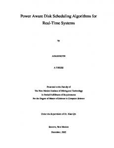
Figure 1: MapReduce framework.

clouds. The bag of MR jobs could be an iterative MR job, a set of independent MR jobs, or a collection of jobs related to some high-level applications such as Hadoop Hive [19]. A MR job at a high level essentially consists of two sets of tasks, map tasks and reduce tasks as shown in Figure 1. The executions of both sets of tasks are synchronized into different stages, sequentially. In the map stage, the entire dataset is partitioned into several smaller chunks in the form of key-value pairs, each chunk being assigned to a map node for partial computation results. The map stage ends up with a set of intermediate key-value pairs on each map node, which are further shuffled based on the intermediate keys into a set of scheduled reduce nodes where the received pairs are aggregated to obtain the final results. For an iterative MR job, the final results could be tentative and further partitioned into a new set of map nodes for the next round of the MR computation. A bag of MR jobs may have multiple stages of MR computation, each stage running either map or reduce tasks in parallel, with enforced synchronization only between them. Therefore, the executions of the jobs can be viewed as a fork&join workflow characterized by multiple synchronized stages, each consisting of a collection of sequential or parallel map/reduce tasks. An example of such a workflow is shown in Figure 2, which is composed of 4 stages, each with 8, 2, 4 and 1 (map/reduce) tasks. These tasks are scheduled on different nodes for parallel execution. In heterogeneous clouds, each node, depending on the performance or the configuration, could have different service rates. As the resources of the Cloud computing are on-demand provisioned according to the typical ”pay-as-you-go” model, the costeffective selection and utilization of the resources for each running task are thus a pragmatic concern of the CSPs to compute their MR workloads, especially the computation budget is fixed. In this paper, we are interested in the cost-effective scheduling of such a bag of MR jobs on a set of heterogeneous (virtual) machines in Clouds, each with different

Figure 2: An example of a 4-stage iterative MapReduce job.

performance and service rates, in an efficient way. We call this scheduling task-level scheduling, which is fine grained compared to the frequently discussed job-level scheduling, where the scheduled unit is a job instead of a task. More specifically, we concern ourselves with the following two optimization problems: 1) Given a fixed budget B, how to efficiently select the machine from a candidate set for each task so that the total scheduling length of the job is shortest without breaking the budget; 2) Given a fixed deadline D, how to efficiently select the machine from a candidate set for each task so that the total monetary cost of the job is lowest without missing the deadline; At the first sight, both problems are primary-dual each other; solving one is sufficient to solve the other. However, we will show that there are still some asymmetries in their solutions. In particular, we focus squarely on the first problem, and briefly discuss the second. To address the first problem, we first design an efficient greedy algorithm for computing the minimum execution time with a given budget for each stage. Based on the structure of this problem and the adopted greedy choice, we further prove the optimality of this algorithm in terms of the execution time and consumed budget. With these results, we further develop a dynamic programming algorithm to achieve a global optimal solution within a time complexity of O(κB 2 ). In contrast, the second problem is relatively straightforward as we can change it into the standard multiple-choice knapsack (MCKS) problem [20] via a parallel transformation. Our results show that the problems can be efficiently solved if the total budget B or the deadline D are polynomially bounded by the number of tasks or the number of stages in the workflow, which is usually the case in practice.

The rest of this paper is organized as follows: in Section II, we introduce some background knowledge regarding to the MR framework and survey some related work. Section III is our problem formulation. The proposed budgetdriven algorithms are presented in Section IV and their empirical studies are in the following Section V. Finally, we conclude the paper in Section VI. II. BACKGROUND

AND

R ELATED W ORK

The MR framework was first advocated by Google in 2004 as a programming model for its internal massive data processing [21]. Since then it has been widely discussed and soon accepted as the most popular paradigm for data intensive processing in different contexts. There are many implementations of this framework in both industry and academia such as Hadoop [22], Dryad [23], Greenplum [24]. As the most popular open source implementation, Hadoop MR has become the de facto research prototype on which many related studies are conducted. Therefore, we use the terminology of the Hadoop community in the rest of this paper, and in particular, most of the related work we overview in this section are built up on the Hadoop implementation. Hadoop MR is made up of an execution runtime and a distributed file system. The execution runtime is responsible for job scheduling and execution, which is composed of one master node called JobTracker and some slave nodes called TaskTrackers. In contrast, the distributed file system, called HDFS, is used to manage task and data across nodes. When the JobTracker receives a submitted job, it first splits the job into a number of map and reduce tasks and then allocates them to the TaskTrackers. As with most distributed systems, the performance of the task scheduler has great impact on the scheduling length of a job, in our particular case, also the budget consumed. Hadoop MR provides a FIFO-based default scheduler at job level while at task level, it provides a TaskScheuler interface, which allows developers to design their own schedulers. By default, each job would occupy the whole cluster and execute in order. To overcome this defect and fairly share the cluster among jobs and users over time, Facebook and Yahoo! leveraged the interface to implement Fair Scheduler [25] and Capacity Scheduler [26], respectively. In addition to fairness, research on the scheduler of Hadoop MR with respect to different opportunities for improving the scheduling policies exists. For instance, Hadoop adopts speculative task scheduling to minimize the slowdown in the synchronization phases caused by straggling tasks in a homogeneous environment [22]. To extend this idea to heterogeneous clusters, Zaharia et al. [18] proposed the LATE algorithm. But their algorithm does not consider the phenomenon of dynamic loading, which is common in practice. This issue was studied by You et al. [14] and they proposed a load-aware scheduler. Another instance is the delay scheduling mechanism which was developed in [12] to

 

t1jl

t2jl

p1jl

p2jl

m

...

tjl jl

...

m pjl jl

 

Table I: Time-price table of task Jjl

improve data locality with relaxed fairness. Apart from these, other research efforts include power-aware scheduling [27], deadline constraint scheduling [28], and scheduling based on automatic task slot assignments [29] to quote a few. Although these results improve different aspects of MR scheduling, they are mostly system performance-centric. It appears that no one yet shares our goal of focusing on the monetary cost of the problem. However, there are some similar studies in the context of scientific workflow scheduling on HPC platforms including the Grid and Cloud [30]–[32]. Yu et al. [30] discussed this problem based on service Grids where a QoS-based workflow scheduling method was presented to minimize the execution cost and yet meet the time constraints imposed by the user. In contrast, Zeng et al. [31] considered the executions of large scale many-task workflows in Clouds with budget constraints. To effectively balances the execution time-and-monetary costs, they proposed ScaleStar, a budget-conscious scheduling algorithm, which assigns the selected task to a virtual machine with higher comparative advantage. Almost at the same time, Caron et al. [32] studied the same problem for non-deterministic workflows. They presented a way of transforming the initial problem into a set of addressed sub-problems thereby proposing two new allocation algorithms for resource allocations under budget constraints. All these studies focus on the scheduling of scientific workflows with a deterministic or non-deterministic DAG (directed acyclic graph) shape. In this sense, in our context, the abstracted fork&join workflow can be viewed as a special case of general workflows. However, our focus is on MR scheduling within budget and deadline constraints, rather than on the general workflow scheduling problem. III. P ROBLEM F ORMULATION We model an iterative MR job as a multi-stage fork&join workflow that consists of κ stages (called κ-stage job), each stage j having a collection of independent map or reduce tasks, denoted as Jj = {Jj0 , Jj1 , ..., Jjnj }, 0 ≤ j < κ, and nj + 1 is the size of stage j. In a cloud platform, each map or reduce task may be associated with a set of machines that are provided by the cloud infrastructure provider to run that task, each depending on the performance, with different charge rates. More specifically, for Task Jjl , 0 ≤ j < κ and 0 ≤ l ≤ nj the available machines and corresponding prices (service rates) are listed in Table I.

Table II: Notation frequently used in model and algorithm descriptions Symbol κ Jji Jj nj n tujl pujl mjl m Bjl B Tjl (Bjl ) Tj (Bj ) T (B) Dj Cjl (Dj ) C(D)

Meaning the number of stages the ith task in stage j task set in stage j the number of tasks in stage j the total number of tasks in the workflow the time to run task Jjl on machine Mu the cost rate for using Mu the total number of the machines that can run Jjl the total size of time-price tables of the workflow the budget used by Jjl the total budget for the MapReduce job the shortest time to finish Jjl given Bjl the shortest time to finish stage j given Bj the shortest time to finish the job given B the deadline to stage j the minimum cost to finish Jjl in stage j within Dj the minimum cost to finish the job within D

In this table, tujl , 1 ≤ u ≤ mjl represents the time to run task Jjl on machine Mu whereas pujl represents the corresponding price for using that machine, and mjl is the total number of the machines that can run Jjl . Here, time is sorted in increasing order and the prices in decreasing order. Without loss generality, we assume that the values of time and prices are unique in their own sequence. This assumption is based on the observation that, when two machines have the same run time for a task, no one will select the expensive one. Similarly, for any two machines with same price, no one will select the slow machine to run a task. Some frequently used symbols are then listed in Table II for quick reference in the following description. 1) Budget Constraints: Given budget Bjl , the shortest time to finish task Jjl , denoted as Tjl (Bjl ), is defined as Tjl (Bjl ) =

tujl

pu+1 jl

m pjl jl ,

< Bjl
← Lookup(Jjl , u − 1, u) u 19: δjl∗ ← pu−1 − p ∗ ∗ jl jl 20: if Bj′ ≥ δjl∗ then ⊲ reduce Jjl∗ ’s time ′ ′ 21: Bj ← Bj − δjl∗ 22: ⊲ Update 23: Bjl∗ ← Bjl∗ + δjl∗ 24: Tjl∗ ← tu−1 jl 25: Mjl∗ ← u − 1 26: else 27: return (Tjl∗ ) 28: end if 29: end while 30: end procedure

The idea of the algorithm is simple. To ensure that all the tasks in stage j have sufficient budget to finish P while mminimizing Tj (Bj ), we first require Bj′ = Bj − l∈[0,nj ] pjl jl ≥ 0 and then iteratively distribute Bj′ in a greedy manner each time to the task whose current execution time determines Tj (Bj ) (i.e., the slowest one). This process continues until no sufficient budget is left over. Algorithm 1 shows the pseudo code of the algorithm. In the algorithm, we use three profile variables Tjl , Bjl and Mjl for each task Jjl in order to record its execution time, assigned budget, and the selected machine (Lines 610). After setting these variables with their initial values, the algorithm enters into its main loop to iteratively update the profile variables associated with the current slowest task (i.e.,Jjl∗ ) (Lines 11-30). By searching the time-price table of Jjl∗ (i.e., Table I), the Lookup function can obtain the costs of the machines indexed by its second and third arguments. Each time the next faster machine (i.e., u − 1) is selected when more δjl∗ is paid. The final distribution information is updated in the profile variables (Line 18-28). Theorem 4.1: Given budget Bj for stage j having nj tasks, Algorithm 1 yields the optimal solution to the distribution of the budget Bj to all the nj tasks in that stage Bj log nj within time O( min0≤l≤n {δjl } + nj ). j

Proof: Given budget Bj to stage j, by following the greedy algorithm, we can obtain a solution ∆j = {b0 , b1 , ..., bnj } where bl is the budget allocated to task Jjl , 0 ≤ l ≤ nj . Based on this sequence, we can further compute the corresponding finish time sequence of the tasks as t0 , t1 , ..., tnj . Clearly, there exists k ∈ [0, nj ] that determines the stage completion time to be Tj (Bj ) = tk Suppose ∆∗j = {b∗0 , b∗1 , ..., b∗nj } is an optimal solution and its corresponding finish time sequence is t∗0 , t∗1 , ..., t∗nj . Given budget Bj , there exists k ′ ∈ [0, nj ] satisfying Tj∗ (Bj ) = t∗k′ . Obviously, tk ≥ t∗k′ . In the following we will show tk = t∗k′ . To this end, we consider two cases: 1) If for ∀l ∈ [0, nj ], t∗l ≤ tl , then we have b∗l ≥ bl . This is impossible because given b∗l ≥ bl for ∀l ∈ [0, nj ], the greedy algorithm would have sufficient budget ≥ b∗k − bk to further reduce tk of taskk , which is contradictory to Tj (Bj ) = tk , unless b∗k = bk , but in this case, Tj∗ (Bj ) will be tk , rather than t∗k (Again, case 1 is impossible). 2) Given the result in 1), there must exist i ∈ [0, nj ] that satisfies ti < t∗i . This indicates that in the process of the greedy choice, taski is allocated budget to reduce the execution time at least from t∗i to ti . In other words, t∗i once determined the stage completion time during the greedy choice process and this happened no later than when Tj (Bj ) = tk . Therefore, we have t∗i ≥ tk ≥ t∗k ≥ t∗i , then tk = t∗k′ . Overall, tk = t∗k′ , that is, the algorithm making the greedy choice at every step produces an optimal solution. The time complexity of this algorithm is straightforward. It consists of the overhead in initialization (Lines 6-10) and the main loop to update the profile variables (Lines 1130). Since the size of Jj is nj , the initialization overhead is O(nj ). If we adopt some advanced data structure to organize Tjl , 0 ≤ l ≤ nj for efficient identification of the slowest task, l∗ can be obtained within O(log nj ) (Line B 12). On the other hand, there are at most O( min0≤l≤nj {δjl } ) j iterations (Line 11). Overall, we have the time complexity Bj log nj of O( min0≤l≤n {δjl } + nj ). j Since all the κ stages can be computed in parallel, the total time complexity for the parallel pre-computation is Bj log nj + nj }). O( max { j∈[0,κ) min0≤l≤nj {δjl } Given Theorem 4.1, we can immediately have the following corollary, which is a direct result of the first case in the proof of Theorem 4.1. Corollary 4.2: Algorithm 1 minimizes the budget to achieve the optimal stage execution time. 2) Global Distribution: Now we consider the second step. Given the results of Algorithm 1 for all the κ stages, we try to obtain a dynamic programming recursion to compute the global optimal result. To this end, we use T (j, r) to represent the minimum total time to complete stages indexed

from j to κ when budget r is available, and have the following recursion (0 < j ≤ κ, 0 < r ≤ B): ( T (j, r) =

min {Tj (nj , q) + T (j + 1, r − q)}

if j < κ

Tj (nj , r)

if j = κ

0