On the Automatic Tuning of PID Type Controllers via the ... - IEEE Xplore

On the Automatic Tuning of PID Type Controllers via the Magnitude Optimum Criterion Konstantinos G. Papadopoulos*, Nikolaos D. Tselepis* and Nikolaos I. Margaris*

*ABB Switzerland Ltd., Department of Medium Voltage Drives, Thrgi, CH-5300, Switzerland *Aristotle University of Thessaloniki, Department of Electrical & Computer Engineering, GR-54124, Greece email: [email protected]*, [email protected]*, [email protected]*

Abstract- The problem of on line tuning the PID controller

used in type-I single input-single output control systems is investigated. This problem is met over many industry applications and involves two basic constraints process model and

2)

1)

the existence of a poor

inability to measure the states of the

process. With respect to these constraints, a systematic method

industries are still tuned manually by control or commissioning engineers and operators. As a result, the tuning is done based on past experiences and heuristics. With respect to the above, the development of a systematic automatic PID tuning procedure has to solve three issues.

for automatic tuning of the PID controller is proposed. The

1) Firstly, such a tuning procedure has to decide the optimal

method is inspired from the well known Magnitude Optimum

PID type controller for the controlled process. In that, it has to decide whether the controlled process needs I or PI control and if the D part has to be added or omitted. 2) Secondly, it is necessary for such a tuning procedure to end up in a control loop which achieves a robust performance in terms of reference tracking and output disturbance rejection. The latter is of great importance especially in the field of electric motor drives where demanding requirements are often met. 3) Thirdly, such a method should consider an adaptive behavior of the controller in case the process model changes rather frequently. In cases when variations of the plant occur, the controller should have the benefit of taking into account such variations and retune its parameters based on the new model of the process.

design criterion. Throughout the investigation, it is shown that the straightforward application of the Magnitude Optimum principle for tuning the PID controller in the ideal case of a known single input-single output linear process model, reveals a feature of the method called 'the preservation of the shape of the step and frequency response' of the final closed-loop control system. This shape is characterized by a specific performance in terms of overshoot (4.47%), settling and rise time of the closed-loop control system. For that reason, the proposed method tunes the PID controller's parameters automatically, so that the step response of the control loop achieves the aforementioned specific performance. For applying the method, an open-loop experiment of the process is carried out which serves for initializing the algorithm. The method proceeds by identifying on line the dominant time constants of the plant and the 'parasitic' one of the closed-loop system. The potential of the proposed method is justified via simulation examples for two process models met in various industry applications.

I.

INTRODUCTION

The effectiveness and efficiency of the PID control algo­ rithm has been widely proved throughout its application to many industrial control problems, [1]. It is by far accepted that the PID control law offers the simplest feasible solution to many real-world control problems, [1]. More than 90% of modern industrial products, are still based around PID algorithms, [1], [7]. The problem of tuning a PID controller involves always two sites. The first site deals with the problem of tuning the PID parameters based on a known process model. The second site deals with the problem of the PID controller's tuning when there is no a priori knowledge regarding the model of the process, [11], [12]. This kind of PID tuning is often called "tuning on demand" or "one shot tuning", [2]. Roughly speaking, as stated in [3], by automatic tuning we mean a method where a controller is tuned automatically on demand from a user. Typically the user will either push a button or send a command to the controller. The problem of automatic tuning of PID controllers seems to have been treated thoroughly according to [1], since many patents have been developed towards this issue. However, as stated in [2], [7], a vast majority of the PID controllers in the

978-1-4673-0342-2112/$3l.00 ©2012 IEEE

In order to develop such a tuning technique, the advantages of the well known Magnitude Optimum criterion [4], will be exploited throughout this work. The Magnitude Optimum criterion, introduced by Sartorius and Oldenbourg [4], [5], is based on the idea of designing a controller, which ren­ ders the magnitude of the closed-loop frequency response as close as possible to unity, in the widest possible frequency range. Oldenbourg and Sartorius applied the Magnitude Op­ timum criterion in type-I systems with stable real poles. The design of control systems with the Magnitude Optimum crite­ rion of Oldenbourg-Sartorius presents at least two important advantages: 1) they do not require the complete plant model [6] and 2) the setpoint response of the closed-loop system is excellent, [7]. However, excluding the German bibliography [8] - [10], the Magnitude Optimum criterion is rarely referred today [5], [6]. This can be justified by the several negative comments that occasionally have been stated in the literature, see [10], [13], [14]. In the sequel it will be shown that the straightforward application of the Magnitude Optimum criterion for tuning the PID controller reveals an attractive feature of the method called 'the preservation of the shape of the step and frequency response' of the final closed-loop. It is shown that, in case of a known process model, the step response of the closed-

869

leIT 2012

2

loop exhibits a specific performance characterized by specific features in terms of overshoot (4.47%), settling and rise time. Motivated by this attractive feature, the proposed method exploits this so called "preservation of the shape" and tunes the PID controller's parameters in such a way so that the specific performance with these specific characteristics is achieved. The proposed method proves promising enough, since in many industry applications, i.e control of electrical drives, the model of the process is normally inaccurate since many model parameters are often unknown or change quite frequently. II.

DIRECT

PID

TUNING BASED ON THE MAGNITUDE

OPTIMUM CRITERION

The closed-loop system of Fig.l is considered, where

r(s), e(s), u(s), y(s), do(s) and di(s) are the reference input,

the control error, the input and output of the plant, the output and the input disturbances respectively. In addition, the real process is described by

1 (1) G (s) = (1 +ST ) (1 +STp2 ) ... (1 +sT ) , PI Pn where Tpl > Tp2 > ... > TPn' This type of modelling is not

restrictive since it will be shown in Section V that the proposed method can be applied in processes with time delay or right half plane zeros. Parameter kp stands for the plant's dc gain. In vector controlled medium voltage drives for example, kp stands for the pulse width modulator's linear gain kpWM which is assumed to remain linear over the whole operating range of the motor. Supposing that little information about the process is available, it is conceived as as a first order one defined by the approximation

1 G (s) = 1 +sh ' p �

(2)

where hp = E�1 TPi is the equivalent sum time constant of the plant. When the information about the plant is limited, the control that can consciously be applied is limited to integral control, so that the system exhibits at least zero steady state position error.

r

y(s)

( s)

y,(s) n,(s) Fig. I. Block diagram of the closed-loop control system. dc gain and kh stands for the feedback path.

Integral control of the approximate plant By applying integral action given by

1 (3) sIiI (1 +sTI:J , to the approximate plant (2), the resulting closed-loop transfer kpC(s)G(s) functIOn T (s) = l+kpk hC(S)G(S) takes the form C(s) =

is the plant's

arising from its implementation. According to the conventional design via the Magnitude Optimum principle, the integration time constant Iii of the controller and the parameter kh in the feedback path will be determined so that IT(jco) I c:::' 1, in the wider possible frequency range. The magnitude of (4) is given by

IT (jco)1

�

. 1f;hC04 + (Iii - 2kpkhh) Iii co2 +k�k�

(5)

IT(jco) I c:::' 1 is satisfied if

kh = 1 and

Iii

=

2kpkhh,

(6)

holds by. In that case, the magnitude takes the form

IT (jco)1

�

1 4Tico4 +l'

(7)

which is close to unity in the low frequency region. Condition

kh = 1 implies that the closed-loop system has zero steady

state position error. In vector controlled electrical motor drives, condition kh = 1 is much critical since in the flux path (d, q components), it stands for the estimator model which calculates Yd, Yq out of the voltage that is finally sent to the motor. Substituting (6) into (4), leads to

1 2Tfs2 +2sh +l' Normalizing the time by setting s' = sTI. leads to 1 T(s,) = 2s'2 +2s' +l' �

T(s) = �

A.

kp

(8)

(9)

At this point it is necessary to declare that by using only the integration time constant Iii and if kh = 1, which results in the above closed-loop dynamic behavior, the sum time constant of the closed-loop system h can be estimated by the relation y;

•

I.esf

=

l 2kpkh

=

Iii

2kp'

(10)

kP B. Integral control of the real plant sIiI (1 +sTI.e) (1 +sTI.p) +khkp If the same control law, (6), is applied to the real plant (1), (4) kp the resulting closed-loop transfer function is given by s2Iilh +sIiI +kpkh T (s' ) = -=------,,-------,,------;-------:-___=_ for which TI.ehp � 01 and TI. = TI.e +TI.p has been considered. stn+l in n Tp 2 E TPiTp . +... +S,3 7:;;;2 Note that he stands for the controller's unmodelled dynamics r. j=1 r. if-j=1 ] ] 2 ' +2S, +2s +1 lOver many industry applications the controller's unmodelled dynamics Tr.c are negligible compared to the plant's unmodelled dynamics Tr.p' he « Tr.p' (11) �

T(� =

[

� �

870

(

)

(

) ].

3

where hlp = Ei= TP i is the parasitic time constant of the plant. 2 Since the plant has a dominant time constant, PI control of the form exact and p=O.9

,/

p

C (s) = y.!T) �

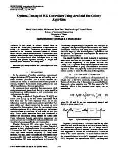
(a) Step responses.

10

'

' 10

U = wfT1

Fi�.�. Comparison of t�e exact and tbe approximate control systems w�tb �ntegral control accordmg to conventional design Magnitude Optimum cntenon.

where again s' = sh. Comparing (9) with (11), it is evident that in the approximate design, the terms of order higher than s, 2 are being neglected in the denominator polynomial. However, these terms have negligible effect on the dynamic behavior of the closed-loop system, because their coefficients are small (they are divided by a power of the closed-loop sum time constant h of higher order). Therefore, the two systems exhibit almost the same dynamic behavior. The accuracy of the approximation depends on the distribution of the plant time pi constants Tpj j = 1, 2, ... n. In cases where ratio p = T r -+ 0, '. . T the accuracy IS especIally satisfactory both in the time and frequency domain, Fig.2. Fig.2(a) presents the step response of the exact and approx­ imate closed-loop system to the reference input r ( s ) and to the output disturbance do (s ) , for two extreme distributions of the plant time constants (p 0.3 and p 0.9). The coincidence of the two responses is especially satisfactory, despite the fact that the determination of parameters �l and kh was based on a crude plant model. Fig.2(b), presents the closed-loop transfer function T (s ) and output sensitivity S(s) = 1 - T (s) frequency responses of the exact and the approximate systems, for the two extreme distributions of the plant time constants (p = 0.3 and p = 0.9). With respect to the above analysis, it is concluded that by using a crude model of the plant and applying only integral control through the conventional design method via the Magnitude Optimum criterion, a closed-loop system with satisfactory response results. The performance features of these response are listed below: • mean rise time tr = 4.40TI: (4.7TI: for p 2: 0.9 and 4.1h for p = 0.3). • mean settling time tss = 7.S6Tr, (S.40h for p 2: 0.9 and 7.32h for p = 0.3). • mean overshoot 4.47% (4.32% for p 2: 0.9 and 4.62% for p = 0.3) • gain margin am = 205d b. • phase margin C/'m = 65.27°. C.

kp (1 +sTn ) . (14) s�Pl (1 +sTPI ) (1 +shl) +khkp (1 +sTn ) For the derivation of (14), we have again set he «T�""Ip and hi = hlp + he = Tr, - Tpl' According to the conventional Magnitude Optimum criterion design, condition ITUro)1 c:::' 1 T(s) =

(b) Closed-loop frequency responses.

=

(13)

is imposed to (12). The resulting closed-loop transfer function is defined by

T"fT,

.2;-0 ------;-----------"o -' "--.:J" T = t/TP1

1 +sTn , S�PI (1 +sTr,e )

=

is satisfied when

(15) (16) (17)

Note that exact zero-pole cancellation occurs in (16), (conven­ tional Magnitude Optimum criterion). Substituting (15)-(17) into (14) results in

T(s) = Setting again s'

=

1 . 2Tfls2 +2hls +1

(IS)

shl leads to 1 2s,2 +2s' +1'

(19)

� � r,les, - Pl - Pl 2kpkh 2kp'

(20)

T(s' )

=

Comparing (19) with (9), it is concluded that with the ap­ plication of PI control via the conventional design of the Magnitude Optimum criterion, a closed-loop system with time and frequency response of the same shape results. However, the response of (19) is faster, because the time scale is smaller (hi < Tr,). In other words, the compensation of the dominant time constant Tpi has left the shape (performance features) of the system time and frequency responses unaltered and produced only a change both in the time and frequency scale respectively. In addition, through the new integration time constant �Pl' with which a step response with mean overshoot 4.47% is achieved, the 'parasitic' time constant of the closed­ loop system can be estimated through the relation y;

_

_

D. Proportional-integral-derivative control If two dominant time constants Tpl, Tp2 of the plant are measured accurately, the transfer function of the process can be approximated by

G( s )

Proportional-integral control

If the dominant time constant Tpi of the plant is evaluated (conventional design method via the Magnitude Optimum criterion), the transfer function process model can be defined by

1, Tpl, 2kpkhTr,1 2kpkh(h - TpJ) = 2kpkh(Tr, - Tn).

kh Tn �Pl

=

1 ( 1 +sTpl ) ( 1 +sTp2 ) ( 1 +sh2 p )'

(21)

( 1 +sTn ) ( 1 +sTv ) S�PID (1 +sTr,e )

(22)

n

where again h2 p = E ,'_ -3 Tr,Pi stands for the parasitic time constant of the plant. Since the plant has two dominant time constants, PID control defined by

(12)

871

C (s) =

4

is imposed to (21). Assuming that Tr,e «Tr,2 and T L2 = T L2p +T Le = Tr, - Tpl - Tp2, the resulting trans r6r function of the closed-loop control system is equal to

T(s)=

[

OW�11"

kp (I +sTn)(1 +sTv) s'liPlD(1 +sTp1)(1 +sTp2)(1 +ST L2)+ khkp (1 +sTn) (1 +sTv)

Condition IT(jm)1

c::::

].

(24)

Tp2,

SIep2

(26)

(a)

(b)

Fig. 3. (a) Typical step response of the process. (b) A series of small step variations of the reference input with alternating sign are imposed for tuning the PID controller's parameters.

2kpkhTr,2= 2kpkh(Tr, - Tpl - TpJ

'liPiD

I

�

T(s)=

2T f2S2+2T L2S +1

.

(28)

Normalizing the time by setting s'= sTr,2 leads to �

T(s,)=

I 2s,2+2s'+I

'

'liPID 'liPiD - 2kpkh - 2kp . _

(30)

PRESERVATION OF THE SHAPE OF TIME AND FREQUENCY RESPONSES

From the analysis presented in Section II it is concluded that, the integration time constant 'lij (j = 0,1,2) , which results via the Magnitude Optimum design criterion, preserves the shape of the system time and frequency responses. The effect of the compensation of some time constants of the plant is limited in the change of the time and frequency scales (speed of response). So, for every time constant distribution of the plant, the design of the controller with the Magnitude Optimum criterion results in closed-loop control systems with the following characteristics: overshoot R::j 4047%, rise time R::j 404TLu, settling time R::j 7.86TLu, where TLu is the ultimate 'parasitic' time constant of the closed-loop system. Of particular interest is the observation that the integration time constant of the controller depends on the 'parasitic' time constant TLu, which is unknown before the implementation and tuning of the closed-loop system. This means that the design of control systems with the Magnitude Optimum design criterion is not based on nominal models, but includes the model uncertainty as a structural element.

TUNING ALGORITHM

The conventional Magnitude Optimum design criterion, presented in Section II, leads effortlessly to the automatic tuning procedure of the controller parameters. The procedure follows the next steps: Step 1: Determination of the gain kp. The gain kp is determined from the step response of the plant at steady state, Fig.3(a). limy (t)= limsG(s) u (s)= kp

l--too

(29)

Comparing (29) with (19) and (9) it becomes evident that with the application of PID control, we end up again, in a closed­ loop system with time and frequency responses of the same shape (performance features), but with even smaller time scale (T L2 < T LI < T L) and consequently even faster. Moreover, with the integration time constant 'liPiD' with which we achieve a step response with 4047% mean overshoot, we can estimate the new 'parasitic' time constant of the closed-loop system using the relation ToL2est

IV. T HE AUTOMATIC

(2 7)

2kpkh(Tr, - Tn - Tv).

Assuming again exact zero-pole cancellation between process poles and controller zeros, see (25)-(2 6), and substituting the control law given by (24)-(27) into (23), results in

III.

0'I5_5.S,,"

,"

(25) Tv

SIep1

ow5_8%

�----------*--+

1 is now satisfied when

1,

kh

(23)

(31)

s--tO

and if the process G(s) is stable. In vector controlled induction motor drives, kp stands for the pulse width modulator gain which is a priori known for the whole operating range of the motor. Moreover, an estimation of the sum time constant Tr, p of the plant can be derived from the step response according to Tr,Pest R::j £..-4sS ' where tss is the settling time of the step response. Then, an auxiliary loop (gray shaded) is placed III the closedloop system of Fig.l, as shown in Figo4. The purpose of this loop is the tuning of the controller Cx(s). The operation of the auxiliary loop is the following. A series of small step variations of the reference input with alternating sign are imposed, so that the plant does not diverge far from its operating point, Fig.3(b). During these variations, the overshoot (undershoot) is being measured and is compared with the reference overshoot (undershoot). According to the preceding analysis Section II, the absolute value of the reference overshoot is 0.0447. The error is fed into a PI controller, which tunes the controller •

y(s)

,(s)

y,(s)

Fig.4. Block diagram of the closed-loop control system and the tuning loop. k is the plant's dc gain and kh stands for the feedback path. ex stands for t&e automatically tuned controller. OVSact is the measured overshoot of y(s) and ovsref is set equal to 4.47%.

872

5

T",,>Tp2 "

" .". .:

)--:-,, ", T", Tnx(k+ 1) then OVSact(k+ 1) < OVSact(k). The same tuning procedure stands for Tvx'

C (s) in succession, so that the overshoot (undershoot) of x the closed-loop step response to be 4.47%. According to the analysis presented in Section II, the controller CAs) is being given the form Cx (s) -

(1 +sTnJ (1 +sTvJ (2kpkhhx - 2kpkhTnx - 2kpkhTvx)s(I+sT!:J

,

(32 )

where hx' Tnx and Tvx are time constants that must be determined automatically. Step 2: Determination of the time constant T!:x' In (32 ) Tnx = Tvx = 0 is set. In succession, a series of step variations on the reference input is imposed and time constant hx is tuned such, so that the overshoot (undershoot) is 4.47%. According to Section II, this will occur when T!:x � T!:. Tuning of T!:x' ( or Iix) is described in Fig.5 Step 3: Determination of the time constant Tnx' With the value of hx given from Step 2, Tvx = 0 is set in (32). Cx (s) -

I�

T = tlTpl

I +sTnx --= _ � _ :.:=. ..,___:_:____=___;_ (2kpkhhx - 2kpkhTnJ s (1 +sT!:c) __ _

(33)

A series of step variations of the reference input is again imposed and Tnx is tuned, so that the overshoot (undershoot) becomes again 4.47%. As shown in Fig.5(a), this will occur when Tnx � Tp1, Section II, PI control. If the 'parasitic' time constant T!: = T!:x - Tnx is relatively large, the procedure can be continu�d by attempting step 4. If the 'parasitic' time constant is sufficiently small, PI control is retained. Step 4: Determination of the time constant Tvx' Given the values of hx and Tnx' Tvx is tuned in such a way, so that the overshoot is again 4.47%, by imposing again a series of step variations on the reference input. As shown in Fig.5(b), this will occur when Tvx � Tp2. If the 'parasitic' time constant T�.Lo2 = T�.Lox - Tnx - Tvx still remains relatively large, a fact that shows that other relatively large time constants may eXIst, the tuning procedure can be continued incorporating in cascade with the controller Cx(s) the necessary number of high-pass stages of the form

(b)

(a)

Fig. 6. Tuning procedure (a) initial conditions differ significan�ly from the nominal ones. (b) initial conditions differ by 10% from the nommal ones.

(34)

where Ta > Tb. For one additional high-pass stage the con­ troller Cx(s) must take the form Cx (s)

=

(1 +sTnJ (1 +sTvx) (1 +sTa) 2kps(T!:x - Tnx - Tvx - Ta) (1 +sT!:c) (1 +sn)

�

( 1 +sTnx) (1 +sTvx) (1 +sTa) 2kps(T!:x - Tnx - Tvx - Ta) (1 +ST!:bc)

(35)

where hbc = T!:c + Tb is considered as the new 'parasitic' time constant of the controller. However, this can only occur if the noise level, that accompanies the controlled physical quantities, allows it. If this is not possible, but the design of a faster closed-loop system is required, then different control techniques should be followed, as cascade control for example [8]. Obviously, the controllers tuning of the inner loops can be achieved using the same procedure. 1) Starting up the procedure: Essentially, no information regarding the plant is required for the starting up the sug­ gested tuning procedure. Consequently, step 1 is not entirely necessary. However, if the gain kp and an estimation of the sum time constant h are known, the first application of the method is acceleratelsignificantly. Moreover, if the gain kp is not known, while the tuning of the controller is being carried out normally, the knowledge of the exact values of the plant time constants is not possible. If in step 2 the initial estimation of T!:x is smaller than T!:, then a significant overshoot occurs. Since a large overshoot is in general undesirable, the procedure must start with an overestimation of h. For the initiation of steps 3 and 4 the initial values of Tnx and Tvx are set equal to T Tn x respectively. Specifically, the convergence of � and r.x � t6e tuning procedure is faster when initially it is Tnx > Tpl and Tvx > Tp2' At this point, it should be noted that, as long as the controller parameters are determined, every repetition of the procedure is faster. In Fig.6 it is shown the application of the suggested tuning procedure when the starting conditions are quite different from the nominal ones. V. A.

•

SIMULATION RESULTS

Process with two dominant time constants For verifying the proposed method a process of the form

G (s')

873

=

0.8435

( 1 +s') ( 1 +0.9s') ( 1 +O.Is') (1 +0. 0 5s ') (1 +0. 02s ' )

(36)

6 2 ,-----�----�--,_--__.

.

1.8 .

k'p =kp(l +0)

1.8 . 1.6 .

1.6

.)vs= 31.5% ovs= 4.47";'..

1.4 1.2 0.8 . 0.8

d;(T)=O.5r(t}

0.6

1---+

0.6 .

d.tr)=O.Sr(t)

'.

0.4

1---+

•

d;(T)=O.25r(t)

. . . L...a. �.. . •. d.(T)=O.25r(t)

0.2 .

0.4 0.2

PID control

PID control

-0.2 L-___L____�____L-___L____�____L-__-' o 50 100 150 200 250 300 350

O L-_____L______�______L-_____L____� o 10 20 30 40 50 T =

T =

tiTp1

Fig. 7. Step response of the closed loop control system after the automatic tuning of the PID controller is finished (black). The process is described by (36) and only Tp1, kp are considered known. During the control loop's operation, the dc gain kp is perturbed by k� = kp(l +a), a = 0.5 while the controller stays tuned with the initial value kp (gray). Overshoot increases from 4.47% --+ 9.2%.

is adopted for which is considered that the approximated model G ( s' ) = (1 kf is known, kp = 0.8435. The automatic +s TpJ ) tuning method ended up to parameters tix = 0.49, tnx = 1.18, tvx = 0.719. All time constants have been normalized according to s' = sTpl' Fig.7, 8. Moreover, for checking the robustness of the proposed tuning method against model parameter varia­ tions an error of the form k� = kp (1+a ) is assumed. In vector controlled induction motor drives, this investigation is of of great importance since kp does not remain constant all over the whole operating range. If a = 0.5, while the controller stays tuned with its nominal value kp, then a change in the overshoot is observed, from 4.47% to 9.2%, Fig.7. Disturbance rejection, remains almost unaltered. B. A

...k'.= kp(l +0)

Fig. 8. Step response of the closed loop control system after the automatic tuning of the PID controller is finished (black). The process is described by (37) and only Tp1, kp are considered known. During the control loop's operation, the dc gain kp is perturbed by k� = kp(1 +a), a = 0.4 while the controller stays tuned with the initial value kp (gray).

VII.

ACKNOWLEDGMENT

This research was performed at the Department of Electrical & Computer Engineering, Aristotle University of Thessaloniki,

Greece and is not a statement by ABB Switzerland Ltd.

non-minimum phase process with time delay

For the non-minimum phase process with time delay four times greater than its dominant time constant 1.3115 (1-0.03s') (1-0.9s') , e- 4s' G (s ) = (I+S') (1+0.81S') (1+0.79S') (1+0.72S') (1+0.41s')

[

tiTp1

1

(37) it has been considered that the approximated model G ( s' ) = (1 +skfTp is known, kp = 1.3115. Variations of parameter kp J) lead to a significant change in the overshoot, output and input disturbance rejection, Fig.8. In this case a = 0.4. Overshoot has increased from 4.4% to 31.5% and settling time has also increased from 36-r to 53.3-r. The same holds also for output disturbance rejection do ( -r). VI. CONCLUSIONS AND OUTLOOK An automatic tuning algorithm for the PID controller's parameters has been presented. The method requires only mea­ surements from an open-loop experiment of the process which serve for initializing the algorithm. The proposed method assumes access to the output of the process and not to the states as it frequently happens in many industry applications.

874

REFERENCES [I] Ang K H., Gregory Chong, Yun Li (1992). "PID Control System Anal­ ysis, Design, and Technology", IEEE Trans. Control Syst. Techno!., vol. 13, No 4, pp. 559-576, 2005. [2] KJ. Astrom, T. Hagglund, e.C Hang, W.K. Ho, "Automatic tuning and adaptation for PID controllers - a survey", Control Engineering Practice, voU, No.4, pp.699-714, 1993. [3] KJ. Astrom, B. Wittenmark, "On self tuning regulators", Automatica, vol.9, pp. 185-199, 1973. [4] Sartorius H., "Die zweckmassige Festlegung der frei wahlbaren Regelungskonstanten", Dissertation, Technische Hochscule, Stuttgart, Germany, 1945. [5] Oldenbourg R.e., Sartorius H., "A Uniform Approach to the Optimum Adjustment of Control Loops", Trans. of the ASME, pp. 1265-1279, 1954. [6] Umland W.1. and Safiuddin M., "Maguitude and Symmetric Optimum Criterion for the Desigu of Linear Control Systems: What Is It and How Does It Compare with the Others?", IEEE Trans. on Industry Applications, vol. 26, No. 3, pp. 489-497, 1990. [7] Astrom K.J. and T. Hagglund, "PID Controllers: Theory, Design and Tuning", Instrument Society of America, 1995. [8] Frohr E, Orttenburger E, "Introduction to Electronic Control Engi­ neering", Berlin: Siemens, 1982. [9] Buxbaum A., Schierau K, Straughen A., "Design of Control Systems for DC Drives", Berlin: Springer-Verlag, 1990. [10] Follinger 0., "Regelungstechnik", Heidelberg: Hiithig, 1994. [II] Guo L., Hung J.Y., Nelms R.M., "Evaluation of DSP-Based PID and Fuzzy Controllers for DC-DC Converters", IEEE Trans. on Ind. Electron., vol. 56, No. 6, pp. 2237-2248, 2009. [12] R. Muszynski, Deskur J., "Damping of Torsional Vibrations in High­ Dynamic Industrial Drives", IEEE Trans. on Ind. Electron., vol. 57, No. 2, pp. 544-552, 2010. [13] Vrancic, D., Strmcnik, S., Juricic D., "A magnitude optimum multiple integration tuning method for filtered PID controller", Automatica, vol. 37, pp. 1473-1479, 2001. [14] Vrancic, D., Peng, Y., Strmcnik, S., "A new PID controller tuning method based on multiple integrations", Control Engineering Practice, vol. 7, pp.623-633, 1999. [15] Papadopoulos KG., Margaris N.J, "Extending the Symmetrical Opti­ mum Criterion to the desigu of PID type-p control loops", Journal of Process Control, Elsevier, vol.22, No I, pp.11-25, 2012.