It turns out that one can lose consistency in generalizing a binary classification method to deal with multiple classes. We study a rich family of multiclass methods ...
On the Consistency of Multiclass Classification Methods by Ambuj Tewari
B.Tech. (Indian Institute of Technology, Kanpur) 2002
A thesis submitted in partial satisfaction of the requirements for the degree of Master of Arts in Statistics in the GRADUATE DIVISION of the UNIVERSITY OF CALIFORNIA, BERKELEY
Committee in charge: Professor Peter L. Bartlett, Chair Professor Bin Yu Professor Stuart J. Russell Fall 2005
The thesis of Ambuj Tewari is approved:
Chair
Date
Date
Date
University of California, Berkeley
Fall 2005
On the Consistency of Multiclass Classification Methods
Copyright 2005 by Ambuj Tewari
1
Abstract
On the Consistency of Multiclass Classification Methods by Ambuj Tewari Master of Arts in Statistics University of California, Berkeley Professor Peter L. Bartlett, Chair
Binary classification is a well studied special case of the classification problem. Statistical properties of binary classifiers, such as consistency, have been investigated in a variety of settings. Binary classification methods can be generalized in many ways to handle multiple classes. It turns out that one can lose consistency in generalizing a binary classification method to deal with multiple classes. We study a rich family of multiclass methods and provide a necessary and sufficient condition for their consistency. We illustrate our approach by applying it to some multiclass methods proposed in the literature.
Professor Peter L. Bartlett Thesis Committee Chair
i
To the memory of my grandfathers, Shri P. C. Tewari & Shri S. S. Dixit.
ii
Contents List of Figures
iii
1 Introduction 1.1 Consistency of Binary Classification Methods . . . . . . . . . . . . . . . . .
1 3
2 Classification Calibration and its Relation to Consistency
6
3 A Characterization of Classification Calibration
17
4 Sufficient Conditions for Classification Calibration
20
5 Examples 5.1 Crammer and Singer . 5.2 Weston and Watkins . 5.3 Lee et al. . . . . . . . 5.4 Another Example with 5.5 Summary of Examples
. . . . . . . . . . . . . . . . . . . . . . . . . . . . . . . . . . . . . . . . . . Sum-to-zero Constraint . . . . . . . . . . . . . .
. . . . .
. . . . .
. . . . .
. . . . .
. . . . .
. . . . .
. . . . .
. . . . .
. . . . .
. . . . .
. . . . .
. . . . .
. . . . .
. . . . .
. . . . .
. . . . .
24 24 25 27 29 30
6 Conclusion
31
Bibliography
32
iii
List of Figures 1.1
The set R for two convex loss functions. . . . . . . . . . . . . . . . . . . . .
4
5.1 5.2
(a) Crammer and Singer (b) Weston and Watkins . . . . . . . . . . . . . . . (a) Lee, Lin and Wahba (b) Loss of consistency in multiclass setting . . . .
25 27
iv
Acknowledgments I am grateful to my advisor, Peter Bartlett, for his guidance and support. Thanks to XuanLong Nguyen and David Rosenberg for useful discussions.
1
Chapter 1
Introduction We consider the problem of classification in a probabilistic setting: n i.i.d. pairs are generated by a probability distribution on X × Y. We think of yi in a pair (xi , yi ) as being the label or class of the example xi . The |Y| = 2 case is referred to as binary classification. A number of methods for binary classification involve finding a real valued function f which minimizes an empirical average of the form 1� Ψyi (f (xi )) . n
(1.1)
i
In addition, some sort of regularization may be used to avoid overfitting. Typically, the sign of f (x) is used to classify an unseen example x. We interpret Ψy (f (x)) as being the loss associated with predicting the label of x using f (x) when the true label is y. An important special case of these methods is that of large margin methods which use {+1, −1} as the set of labels and φ(yf (x)) as the loss. Here φ is some function chosen by taking into account both computational and statistical issues. Bayes consistency of these methods has been analyzed in the literature [4, 6, 13, 9, 1]. In this thesis, we investigate the consistency of
2 multiclass (|Y| ≥ 2) methods which try to generalize (1.1) by replacing f with a vector function f . This category includes the methods of [2, 5, 10] and [11]. Zhang [11, 12] has already initiated the study of these methods. Under suitable conditions, minimizing (1.1) over a sequence of function classes also approximately minimizes the “Ψ-risk” RΨ (f ) = EX Y [ Ψy (f (x)) ]. However, our aim in classification is to find a function f whose probability of misclassification R(f ) (often called the “risk” of f ) is close to the minimum possible (the so called Bayes risk R∗ ). Thus, it is natural to investigate the conditions which guarantee that if the Ψ-risk of f gets close to the optimal then the risk of f also approaches the Bayes risk. If this happens, we say that the classification method based on Ψ is Bayes consistent. Bartlett et al. [1] defined the notion of “classification calibration” to obtain such conditions for binary classification. The authors also gave a simple characterization of classification calibration for convex loss functions. In Chapter 1.1 below, we provide a different point of view for looking at classification calibration for binary classification in order to motivate our geometric approach to multiclass classification. The rest of the thesis is organized as follows. Chapter 2 defines classification calibration in the setting of multiclass classification and provides a justification, in the form of Theorem 2, for studying it: classification calibration is equivalent to Bayes consistency. The main result in Chapter 3 is Theorem 8 which characterizes classification calibration in terms of geometric properties of some sets associated with the loss function Ψ. In Chapter 4, we provide certain sufficient conditions for classification calibration. These are provided with the hope that, in practice, some of these conditions will hold and checking the full condition
3 of Theorem 8 can be avoided. Chapter 5 applies the results obtained in earlier chapters to examine the consistency of a few multiclass methods. Interestingly, many seemingly natural generalizations of binary methods do not lead to consistent multiclass methods. Chapter 6 provides the conclusion.
1.1
Consistency of Binary Classification Methods If we have a convex loss function φ : R �→ [0, ∞) which is differentiable at 0 and
φ� (0) < 0, then it is known [1] that any minimizer f ∗ of EX Y [ φ(yf (x)) ] = EX [ EY|x [ φ(yf (x)) ] ]
(1.2)
yields a Bayes consistent classifier, i.e. P (Y = +1|X = x) > 1/2 ⇒ f ∗ (x) > 0 and P (Y = −1|X = x) < 1/2 ⇒ f ∗ (x) < 0. In order to motivate the approach of the next chapter let us work with a few examples. Let us fix an x and denote the two conditional probabilities by p+ and p− . We also omit the argument in f (x). We can then write the inner conditional expectation in (1.2) as p+ φ(f ) + p− φ(−f ) . We wish to find an f which minimizes the expression above. If we define the set R ∈ R2 as R = {(φ(f ), φ(−f )) : f ∈ R} ,
(1.3)
then the above minimization can be written as min �p, z� z∈R
where p = (p+ , p− ).
(1.4)
4 4
4
3
3
2
2
1
1
-1
1 p� � p�
2
3
4
-1
1
p� � p�
-1
P
2
3
L1
4 L2
-1
(a) Squared Hinge Loss
(b) Inconsistent case
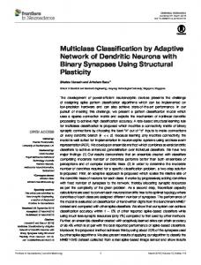
Figure 1.1: The set R for two convex loss functions. The set R is shown in Figure 1.1 (a) for the squared hinge loss function φ(t) = ((1 − t)+ )2 . Geometrically, the solution to (1.4) is obtained by taking a line whose equation is �p, z� = c and then sliding it (by varying c) until it just touches R. It is intuitively clear from the figure that if p+ > p− then the line is inclined more towards the vertical axis and the point of contact is above the angle bisector of the axes. Similarly, if p+ < p− then the line is inclined more towards the horizontal axis and the point is below the bisector. This means that sign(φ(−f ) − φ(f )) is a consistent classification rule which, because φ is a decreasing function, is equivalent to sign(f − (−f )) = sign(f ). In fact, the condition φ� (0) < 0 is not necessary for the existence of a consistent classification rule based on f . For example, if we had the function φ(t) = ((1 + t)+ )2 , we would still get the same set R but will need to change the classification rule to sign(−f ) in order to preserve consistency. Why do we need differentiability of φ at 0? Figure 1.1 (b) shows the set R for a convex loss function which is not differentiable at 0. In this case, both lines L1 and L2 touch R at P but L1 has p+ > p− while L2 has p+ < p− . Thus we cannot create a consistent
5 classifier based on this loss function. The crux of the problem seems to lie in the fact that there are two distinct supporting lines to the set R at P and that these two lines are inclined towards different axes. It seems from the figures that as long as R is symmetric about the angle bisector of the axes, all supporting lines at a given point are inclined towards the same axis except when the point happens to lie on the angle bisector. To check for consistency, we need to examine the set of supporting lines only at that point. In case the set R is generated as in (1.3), this boils down to checking the differentiability of φ at 0. In the following chapters, we will deal with cases when the set R is generated in a more general way and the situation possibly involves more than two dimensions. The intuition developed for the binary case will be proven correct by Propositions 9 and 10 in Chapter 4.
6
Chapter 2
Classification Calibration and its Relation to Consistency Suppose we have K ≥ 2 classes. For y ∈ {1, . . . , K}, let Ψy be a continuous function from RK to R+ = [0, ∞). Let F be a class of vector functions f : X �→ RK . Let {Fn } be a sequence of function classes such that each Fn ⊆ F. Suppose ˆfn is a classifier ˆΨ learned from data. For example, we might obtain ˆfn by minimizing the empirical Ψ-risk R over the class Fn , n
� ˆfn = arg min R ˆ Ψ (f ) = arg min 1 Ψyi (f (xi )) . n f ∈Fn f ∈Fn
(2.1)
i=1
There might be some constraints on the set of vector functions in the class F. For example, a common constraint is to have the components of f sum to zero. More generally, let us assume there is some set C ∈ RK such that F = {f : ∀x, f (x) ∈ C }.
(2.2)
7 Let Ψ(f (x)) denote the vector (Ψ1 (f (x)), . . . , ΨK (f (x)))T . We predict the label of a new example x to be pred(Ψ(f (x))) for some function pred : RK �→ {1, . . . , K}. The Ψ-risk of a function f is RΨ (f ) = EX Y [ Ψy (f (x)) ] , and we denote the least possible Ψ-risk by ∗ = inf RΨ (f ) . RΨ f ∈F
In a classification task, we are more interested in the risk of a function f , R(f ) = EX Y [ 1[pred(Ψ(f (x))) �= Y ] ] , which is the probability that f leads to an incorrect prediction on a labeled example drawn from the underlying probability distribution. The least possible risk is R∗ = EX [ 1 − max py (x) ] , y
where py (x) = P (Y = y | X = x). If ˆfn is the empirical Ψ-risk minimizer then, under ∗ (in probability). It would suitable conditions, one would expect RΨ (ˆfn ) to converge to RΨ
be nice if that made R(ˆfn ) converge to R∗ (in probability). Theorem 2 below states that classification calibration, a notion that we will soon define, is both necessary and sufficient for this to happen. In order to understand the behavior of approximate Ψ-risk minimizers, let us write RΨ (f ) as EX Y [ Ψy (f (x)) ] = EX [ EY|x[ Ψy (f (x)) ] ] . The above minimization problem is equivalent to minimizing the inner conditional expectation for each x ∈ X . Let us fix an arbitrary x for now, so we can write f instead of f (x), py
8 instead of py (x), etc. The minimum might not be achieved and so we consider the infimum1 inf f ∈C
� y
py Ψy (f ) of the conditional expectation above. Define the subsets R and S of RK +
as R = {(Ψ1 (f ), . . . , ΨK (f )) : f ∈ C} , S = conv(R) = conv{(Ψ1 (f ), . . . , ΨK (f )) : f ∈ C} .
(2.3)
We then have inf
f ∈C
� y
py Ψy (f ) = inf �p, Ψ(f )� f ∈C
= inf �p, z�
(2.4)
z∈R
= inf �p, z� , z∈S
where p = (p1 , . . . , pK ). The last equality holds because for a fixed p, the function z �→ �p, z� is a linear function and hence we do not change the infimum by taking the convex hull2 of R. Let us define a symmetric set to be one with the following property: if a point z is in the set then so is any point obtained by interchanging any two coordinates of z. We assume that R is symmetric. This assumption holds whenever the loss function treats all classes equivalently. Note that our assumption about R implies that S too is symmetric. We now define classification calibration of S. The definition intends to capture the property that, for any p, minimizing �p, z� over S leads one to z’s which enable us to figure out the index of (one of the) maximum coordinate(s) of p. Since py and Ψy (f ) are both non-negative, the objective function is bounded below by 0 and hence the existence of an infimum is guaranteed. 2 If z is a convex combination of z(1) and z(2) , then �p, z� ≥ min{�p, z(1) �, �p, z(2) �}. 1
9 Definition 1. A set S ⊆ RK + is classification calibrated if there exists a predictor function pred : RK �→ {1, . . . , K} such that ∀p ∈ ∆K ,
inf
z∈S : ppred(z) inf �p, z� , z∈S
(2.5)
where ∆K is the probability simplex in RK . The following theorem tells us that classification calibration is indeed the right property to study, as it is both necessary and sufficient for convergence of Ψ-risk to the optimal Ψ-risk to imply convergence of risk to the Bayes risk. Theorem 2. Let Ψ be a (vector-valued) loss function and C be a subset of RK . Let F and S be as defined in (2.2) and (2.3) respectively. Then S is classification calibrated iff the following holds. Whenever {Fn } is a sequence of function classes (where Fn ⊆ F and ∪Fn = F) such that ˆfn ∈ Fn and P is the data generating probability distribution, P ∗ RΨ (ˆfn ) → RΨ
implies P R(ˆfn ) → R∗ .
Before we prove the theorem, we need the following lemma. Lemma 3. The function p �→ inf z∈S �p, z� is continuous on ∆K . Proof. Let {p(n) } be a sequence converging to p. If B is a bounded subset of RK , then �p(n) , z� → �p, z� uniformly over z ∈ B and therefore inf �p(n) , z� → inf �p, z� .
z∈B
z∈B
10 Let Br be a ball of radius r in RK . Then we have inf �p(n) , z� ≤ inf �p(n) , z� → inf �p, z�
z∈S
S∩Br
S∩Br
Therefore lim sup inf �p(n) , z� ≤ z∈S
n
inf �p, z� .
z∈S∩Br
Letting r → ∞, we get lim sup inf �p(n) , z� ≤ inf �p, z� . n
z∈S
(2.6)
z∈S
Without loss of generality, assume that for some j, 1 ≤ j ≤ K we have p1 , . . . , pj > 0 and pj+1 , . . . , pK = 0. For all sufficiently large integers n and a sufficiently large ball BM ⊆ Rj we have inf �p, z� = inf
z∈S
z∈S (j)
inf �p(n) , z� ≥ inf
z∈S
z∈S (j)
j � y=1 j � y=1
py zy =
inf
z∈S (j) ∩BM
p(n) y zy =
j �
py zy ,
y=1
inf
z∈S (j) ∩BM
j � y=1
p(n) y zy .
and thus lim inf inf �p(n) , z� ≥ inf �p, z� . n
z∈S
z∈S
(2.7)
Combining (2.6) and (2.7), we get inf �p(n) , z� → inf �p, z� .
z∈S
z∈S
Proof (of Theorem 2). (‘only if’) Suppose we could prove that ∀� > 0, ∃δ > 0 such that ∀p ∈ ∆K , max py − ppred(z) ≥ � ⇒ �p, z� − inf �p, z� ≥ δ . y
z∈S
(2.8)
11 Using this it immediately follows that ∀�, H(�) > 0 where H(�) =
inf
p∈∆K ,z∈S
{�p, z� − inf �p, z� : max py − ppred(z) ≥ �} . y
z∈S
A result of Zhang [12, Corollary 26] then guarantees there exists a concave function ξ on [0, ∞) such that ξ(0) = 0 and ξ(δ) → 0 as δ → 0+ and ∗ ). R(f ) − R∗ ≤ ξ(RΨ (f ) − RΨ P P ∗ easily gives R(ˆ This inequality combined with RΨ (ˆfn ) → RΨ fn ) → R∗ . We now prove the
implication in (2.8) by contradiction. Suppose S is classification calibrated but there exists � > 0 and a sequence (z(n) , p(n) ) such that (n)
ppred(z(n) ) ≤ max p(n) y −�
(2.9)
y
and
� �p
(n)
,z
(n)
� − inf �p
(n)
z∈S
� , z� → 0 .
Since p(n) come from a compact set, we can choose a convergent subsequence (which we still denote as {p(n) }) with limit p. Using Lemma 3, we get �p(n) , z(n) � → inf �p, z� . z∈S
As before, we assume that precisely the first j coordinates of p are non-zero. Then the first j coordinates of z(n) are bounded for sufficiently large n. Hence lim sup�p, z(n) � = lim sup n
n
j � y=1
(n) (n) (n) p(n) , z � = inf �p, z� . y zy ≤ lim �p n→∞
Now (2.15) and (2.9) contradict each other since p(n) → p.
z∈S
12 (‘if’) If S is not classification calibrated then by Theorem 8 and Propositions 9 and 10, we have a point in the boundary of some S (i) where there are at least two normals and which does not have a unique minimum coordinate. Such a point should be there in the projection of R even without taking the convex hull. Therefore, we must have a sequence z(n) in R such that δn = �p, z(n) � − inf �p, z� → 0
(2.10)
ppred(z(n) ) < max py .
(2.11)
z∈S
and for all n, y
Without loss of generality assume that δn is a monotonically decreasing sequence. Further, assume that δn > 0 for all n. This last assumption might be violated but the following proof then goes through for δn replaced by max(δn , 1/n). Let gn be the function that maps every x to one of the pre-images of z(n) under Ψ. Define Fn as Fn = {gn } ∪ (F ∩ {f : ∀x, �p, Ψ(f (x)� − inf �p, z� > 4δn } z∈S
∩ {f : ∀x, ∀j, |Ψj (f (x)| < Mn }) where Mn ↑ ∞ is a sequence which we will fix later. Fix a probability distribution P with arbitrary marginal distribution over x and let the conditional distribution of labels be p for all x. Our choice of Fn guarantees that the Ψ-risk of gn is less than that of other elements of Fn by at least 3δn . Suppose, we make sure that � �� � � �ˆ P n �R Ψ (gn ) − RΨ (gn )� > δn → 0 , � P
n
sup f ∈Fn −{gn }
� � � �ˆ �RΨ (f ) − RΨ (f )� > δn
(2.12)
→0.
(2.13)
13 ∗ which implies that Then, with probability tending to 1, ˆfn = gn . By (2.10), RΨ (gn ) → RΨ ∗ in probability. Similarly, (2.11) implies that R(ˆ fn ) � R∗ in probability. RΨ (ˆfn ) → RΨ
We only need to show that we can have (2.12) and (2.13) hold. For (2.12), we apply Chebyshev inequality and use a union bound over the K labels to get � �� � K 3 �z(n) � � �ˆ ∞ P n �R (g ) − R (g ) > δ � Ψ n Ψ n n ≤ 4nδn2 The right hand side can be made to go to zero by repeating terms in the sequence {z(n) } to slow down the rate of growth of �z(n) �∞ and the rate of decrease of δn . For (2.12), we use standard covering number bounds (e.g. see[7, Section II.6]). � P
n
sup f ∈Fn −{gn }
� � � �ˆ �RΨ (f ) − RΨ (f )� > δn
� ≤ 8 exp
nδn2 64Mn2 log(2n + 1) − δn2 128Mn2
�
Thus Mn /δn needs to grow slowly enough such that nδn4 →∞. Mn4 log(2n + 1)
The definition of classification calibration as stated above is not concrete enough to be of any use in checking the consistency of a multiclass method corresponding to a given loss function. We now study the property of classification calibration with the aim of arriving at a characterization expressed in terms of concretely verifiable properties of the loss function. Before we do that, let us observe that it is easy to reformulate the definition in terms of sequences. The exact statement of the reformulation is provided by the following lemma whose proof, being entirely straightforward, is omitted.
14 (n) } in S Lemma 4. S ⊆ RK + is classification calibrated iff ∀p ∈ ∆K and all sequences {z
such that �p, z(n) � → inf �p, z� ,
(2.14)
ppred(z(n) ) = max py
(2.15)
z∈S
we have y
ultimately. This makes it easier to see that if S is classification calibrated then we can find a predictor function such that any sequence achieving the infimum in (2.4) ultimately predicts the right label (the one having maximum probability). The following lemma shows that symmetry of our set S allows us to reduce the search space of predictor functions (namely to those functions which map z to the index of a minimum coordinate). Lemma 5. If there exists a predictor function pred satisfying condition (2.5) in the definition of classification calibration (Definition 1), then any predictor function pred� satisfying ∀z ∈ S, zpred� (z) = min zy y
(2.16)
also satisfies (2.5). Proof. Consider some p ∈ ∆K and a sequence {z(n) } such that (2.14) holds. We have ppred(z(n) ) = maxy py ultimately. In order to derive a contradiction, assume that ppred� (z(n) ) < maxy py infinitely often. Since there are finitely many labels, this implies that there is a
15 subsequence {z(nk ) } and labels M and m such that the following hold, pred(z(nk ) ) = M ∈ {y � : y � = max py } , y
pred� (z(nk ) ) = m ∈ {y � : y � < max py } , y
�p, z(nk ) � → inf �p, z� . z∈S
(n )
(n )
˜ and z˜ denote the vectors obtained from Because of (2.16), we also have zM k ≥ zm k . Let p p and z respectively by interchanging the M and m coordinates. Since S is symmetric, z∈S⇔˜ z ∈ S. There are two cases depending on whether the inequality in � � (n ) (nk ) ≥0 lim inf zM k − zm k
is strict or not. (n )
(n )
If it is strict, denote the value of the lim inf by � > 0. Then zM k − zm k > �/2 ultimately and hence we have (n )
(nk ) ) > (pM − pm )�/2 �p, z(nk ) � − �p, z˜(nk ) � = (pM − pm )(zM k − zm
for k large enough. This implies lim inf�p, z˜(nk ) � < inf z∈S �p, z�, which is a contradiction. (n )
(n )
Otherwise, choose a subsequence3 {z(nk ) } such that lim(zM k − zm k ) = 0. Multiplying this with (pM − pm ), we have lim
k→∞
� � p, z(nk ) � = 0 . �˜ p, ˜z(nk ) � − �˜
We also have ˜� = inf �˜ ˜(nk ) � = lim�p, z(nk ) � = inf �p, z� = inf �˜ p, z p, z� , lim�˜ p, z z∈S
3
We do not introduce additional subscripts for simplicity.
z∈S
z∈S
16 where the last equality follows because of symmetry. This means �˜ p, z(nk ) � → inf �˜ p, z� z∈S
and therefore p˜pred(z(nk ) ) = pM ultimately. This is a contradiction since p˜pred(z(nk ) ) = p˜M = pm . Having identified the class of potentially useful predictor functions, we will henceforth assume that pred is defined as in (2.16).
17
Chapter 3
A Characterization of Classification Calibration We give a characterization of classification calibration in terms of normals to the convex set S and its projections onto lower dimensions. For a point z ∈ ∂S, we say p is a normal to S at z if1 �z� − z, p� ≥ 0 for all z� ∈ S. Define the set of positive normals at z as N (z) = {p : p is a normal to S at z} ∩ ∆K . Definition 6. A convex set S ⊆ RK + is admissible if ∀z ∈ ∂S, ∀p ∈ N (z), we have argmin(z) ⊆ argmax(p)
(3.1)
where argmin(z) = {y � : zy� = miny zy } and argmax(p) = {y � : py� = maxy py }. (n) } Lemma 7. If S ⊆ RK + is admissible then for all p ∈ ∆K and all bounded sequences {z
such that �p, z(n) � → inf z∈S �p, z�, we have ppred(z(n) ) = maxy py ultimately. 1
Our sign convention is opposite to the usual one (see, for example, [8]) because we are dealing with minimum (instead of maximum) problems.
18 Proof. Let Z(p) = {z ∈ ∂S : p ∈ N (z)}. Taking the limit of a convergent subsequence of the given bounded sequence gives us a point in ∂S which achieves the infimum of the inner product with p. Thus, Z(p) is not empty. It is easy to see that Z(p) is closed. We claim that for all � > 0, dist(z(n) , Z(p)) < � ultimately. For if we assume the contrary, boundedness implies that we can find a convergent subsequence {z(nk ) } such that ∀k, dist(z(nk ) , Z(p)) ≥ �. Let z∗ = limk→∞ z(nk ) . Then �p, z∗ � = inf z∈S �p, z� and so z∗ ∈ Z(p). On the other hand, dist(z∗ , Z(p)) ≥ � which gives us a contradiction and our claim is proved. Further, there exists �� > 0 such that dist(z(n) , Z(p)) < �� implies argmin(z(n) ) ⊆ argmin(Z(p))2 . Finally, by admissibility of S, argmin(Z(p)) ⊆ argmax(p) and so argmin(z(n) ) ⊆ argmax(p) ultimately. The next theorem provides a characterization of classification calibration in terms of normals to S. Theorem 8. Let S ⊆ RK + be a symmetric convex set. Define the projections S (i) = {(z1 , . . . , zi )T : z ∈ S} for i ∈ {2, . . . , K}. Then S is classification calibrated iff each S (i) is admissible. Proof. We prove the easier ‘only if’ direction first. Suppose some S (i) is not admissible. / Then there exist z ∈ ∂S (i) and p ∈ N (z) and a label y � such that y � ∈ argmin(z) and y � ∈ argmax(p). Choose a sequence {z(n) } converging to z. Modify the sequence by replacing, in each z(n) , the coordinates specified by argmin(z) by their average. The resulting sequence is still in S (i) (by symmetry and convexity) and has argmin(z(n) ) = argmin(z) ultimately. 2
For a set Z, argmin(Z) denotes ∪z∈Z argmin(z).
19 Therefore, if we set pred(z(n) ) = y � , we have ppred(z(n) ) < maxy py ultimately. To get a sequence in S look at the points whose projections are the z(n) ’s and pad p with K − i zeros. To prove the other direction, assume each S (i) is admissible. Consider a sequence {z(n) } with �p, z(n) � → inf z∈S �p, z� = L. Without loss of generality, assume that for some j, 1 ≤ j ≤ K we have p1 , . . . , pj > 0 and pj+1 , . . . , pK = 0. We claim that there (n)
exists an M < ∞ such that ∀y ≤ j, zy
(n)
≤ M ultimately. Since pj zj
≤ L + 1 ultimately,
M = max1≤y≤j {(L + 1)/py } works. Consider a set of labels T ⊆ {j + 1, . . . , K}. Consider the subsequence consisting of those z(n) for which zy ≤ M for y ∈ {1, . . . , j}∪T and zy > M for y ∈ {j + 1, . . . , K} − T . The original sequence can be decomposed into finitely many such subsequences corresponding to the 2(K−j) choices of the set T . Fix T and convert the corresponding subsequence into a sequence in S (j+|T |) by dropping the coordinates belonging ˜ be (p1 , . . . , pj , 0, . . . , 0)T . We to the set {j + 1, . . . , K}. Call this sequence z˜(n) and let p have a bounded sequence with ˜(n) � → �˜ p, z
inf
˜ z∈S (j+|T |)
�˜ p, ˜z� .
Thus, by Lemma 7, we have p˜pred(˜z(n) ) = maxy p˜y = maxy py ultimately. Since we dropped only those coordinates which were greater than M , pred(˜ z(n) ) picks the same coordinate as ˜(n) was obtained. Thus we have ppred(z(n) ) = pred(z(n) ) where z(n) is the element from which z maxy py ultimately and the theorem is proved.
20
Chapter 4
Sufficient Conditions for Classification Calibration In this chapter, we prove some propositions that reduce the work involved in checking classification calibration of sets. We will see that the assumptions made in the propositions are often satisfied. Our first proposition states that in the presence of symmetry, points having a unique minimum coordinate can never destroy admissibility. Proposition 9. Let S ⊆ RK + be a symmetric convex set, z a point in the boundary of S and p ∈ N (z). Then argmin(z) ⊆ argmax(p) whenever | argmin(z)| = 1. ˜ obtained from z by interchanging the y, y � coordinates. It also is a point Proof. Consider z in ∂S by symmetry and thus convexity implies zm = (z + ˜z)/2 ∈ S ∪ ∂S. Since p ∈ N (z), �z� − z, p� ≥ 0 for all z� ∈ S. Taking limits, this inequality also holds for z� ∈ S ∪ ∂S. z − z)/2, p� ≥ 0 which simplifies to (zy� − zy )(py − py� ) ≥ 0. Substituting zm for z� , we get �(˜ Thus zy < zy� implies py ≥ py� . Therefore, if | argmin(z)| = 1 and zy = miny� zy� then
21 py ≥ py� for all y � , and so argmin(z) ⊆ argmax(p). If the set S possesses a unique normal at every point on its boundary then the next proposition guarantees admissibility. Proposition 10. Let S ⊆ RK + be a symmetric convex set, z a point in the boundary of S and N (z) = {p} is a singleton. Then argmin(z) ⊆ argmax(p). Thus, S is admissible if |N (z)| = 1 for all z ∈ ∂S. Proof. We will assume that there exists a y, y ∈ argmin(z), y ∈ / argmax(p) and deduce that there are at least 2 elements in |N (z)| to get a contradiction. Let y � ∈ argmax(p). From the proof of Proposition 9 we have (zy� − zy )(py − py� ) ≥ 0 which implies zy� ≤ zy since py − py� < 0. But we already know that zy ≤ zy� and so zy = zy� . Symmetry of S now ˜ ∈ N (z) where p ˜ is obtained from p by interchanging the y, y � coordinates. implies that p ˜ �= p which means |N (z)| ≥ 2. Since py �= py� , p Theorem 8 provides a characterization of classification calibration in terms of admissibility of the projections S (k) . As we will see in the examples later, proving that a certain set is not classification calibrated simply involves finding a projection S (k) and a “bad” point in S (k) violating the condition of admissibility. On the other hand, the characterization is not so easy to use when we wish to assert, rather than deny, classification calibration. The following lemma shows that under certain assumptions we can ignore the projections S (k) and only check the admissibility of S. That we cannot always ignore projections will become clear when we consider examples in the next chapter. Recall that R is the set of points (Ψ1 (f ), . . . , ΨK (f )) as f ranges over C. Define
22 the projections R(k) in the same way as S (k) . Since the operations of taking projections and convex hulls commute, it is easy to see that conv(R(k) ) = S (k) . Theorem 11. If R(k) is closed and S is symmetric and admissible then S (k) is also admissible. Furthermore, if each R(k) is closed and S is also convex then S is classification calibrated. Proof. We only need to prove that R(k) closed and S admissible implies S (k) is admissible since the rest follows from Theorem 8. Suppose R(k) is closed and S (k) is not admissible. Therefore, there exists positive normal p to S (k) at a point z in the boundary of S (k) with argmin(z) �⊆ argmax(p) .
(4.1)
We claim that it is a limit point of R(k) . If not, there is a ball centered at z containing no point of R(k) . This would mean that the infimum of �p, z� over R(k) is strictly less than the infimum over S (k) but this is impossible as conv(R(k) ) = S (k) . Now, since R(k) is closed, z be the point in R such that z = proj(˜ z) where proj is projection operator z ∈ R(k) . Let ˜ mapping (z1 , . . . , zK ) to (z1 , . . . , zk ). Since R ⊆ S, this gives us ˜z ∈ S. Moreover, p˜ is a ˜ is p padded with K − k zeros. This is because normal to S at ˜ z where p �˜ p, z� − ˜z� = �p, proj(z� ) − z� ≥ 0 , z) �⊆ argmax(˜ p), which will give us a contrafor all z� ∈ S. We now claim that argmin(˜ ˜ is p padded with zeros, argmax(˜ diction as S was assumed to be admissible. Since p p) = argmax(p). Also, argmin(˜ z) ⊆ argmin(z) for otherwise applying a suitable permutation to ˜ will give a point ˆz with �p, proj(ˆ the coordinates of z z)� < �p, z�. The claim now follows from (4.1).
23 We will now provide a sufficient condition for R(k) to be closed. To state it, we need the following definition. Definition 12. Let C ⊆ RK be a set and Ψ : C �→ RK + be a loss function. Further, let Ψ(k) = (Ψ1 , . . . , Ψk ) be Ψ restricted to the first k coordinates. The mapping Ψ(k) is boundedly invertible iff for all M > 0, there is an M � > 0 such that �z� ≤ M , z ∈ R(k) implies there is g ∈ C with �g� ≤ M � and Ψ(k) (g) = z. Ψ(k) boundedly invertible roughly means that it has an inverse carrying bounded points in its range to bounded points in the domain. Lemma 13. Suppose that C is closed and Ψ is continuous. If Ψ(k) is boundedly invertible then R(k) is closed. Proof. Suppose z(n) ∈ R(k) and z(n) → z. Then these is an M > 0 such that �z(n) � ≤ M for all n. Bounded invertibility implies there is a sequence {g(n) } such that, for all n, g(n) ∈ C, �g(n) � < M � and (Ψ1 (g(n) ), . . . , Ψk (g(n) )) = z(n) . Being bounded, {g(n) } has a convergent subsequence {g(nk ) }. Since C is closed, the limit g∗ ∈ C. Now, (Ψ1 (g∗ ), . . . , Ψk (g∗ )) = lim (Ψ1 (g(nk ) ), . . . , Ψk (g(nk ) )) (Ψ is continuous) n→∞
= lim z(nk ) n→∞
=z and so z ∈ R(k) .
24
Chapter 5
Examples We apply the results of the previous chapter to examine the consistency of several multiclass methods. In all these examples, the functions Ψy (f ) are obtained from a single real valued function ψ : RK + �→ R as follows Ψy (f ) = ψ(fy , f1 , . . . , fy−1 , fy+1 , . . . , fK ) Moreover, the function ψ is symmetric in its last K − 1 arguments, i.e. interchanging any two of the last K − 1 arguments does not change the value of the function. This ensures that the set S is symmetric. We assume that we predict the label of x to be arg miny Ψy (f ).
5.1
Crammer and Singer The method of Crammer and Singer [3] corresponds to φ(fy − fy� ), C = RK Ψy (f ) = max � y �=y
25
(a)
(b)
Figure 5.1: (a) Crammer and Singer (b) Weston and Watkins with φ(t) = (1 − t)+ . For K = 3, the boundary of S is shown in Figure 5.1(a). At the point z = (1, 1, 1), all of these are normals: (0, 1, 1), (1, 0, 1), (1, 1, 0). Thus, there is no y � such that py� = maxy py for all p ∈ N (z). The method is therefore inconsistent. Even if we choose an everywhere differentiable convex φ with φ� (0) < 0, the three normals mentioned above are still there in N (z) for z = (φ(0), φ(0), φ(0)). Therefore the method still remains inconsistent.
5.2
Weston and Watkins The method of Weston and Watkins [10] corresponds to Ψy (f ) =
�
φ(fy − fy� ), C = RK
(5.1)
y � �=y
with φ(t) = (1 − t)+ . For K = 3, the boundary of S is shown in Figure 5.1(b). The central hexagon has vertices (in clockwise order) (1, 1, 4), (0, 3, 3), (1, 4, 1), (3, 3, 0), (4, 1, 1) and (3, 0, 3). At z = (1, 1, 4), we have the following normals: (1, 1, 0), (1, 1, 1), (2, 3, 1),
26 (3, 2, 1) and there is no coordinate which is maximum in all positive normals. The method is therefore inconsistent. Now assume that φ is a positive convex classification calibrated loss function (i.e. φ� (0) exists and is negative). Note that if φ does not satisfy this assumption then we do not get a consistent method even in the binary classification case. Further assume that φ achieves its minimum. The following proposition then guarantees that Ψ(k) is boundedly invertible for k > 1 and we can ignore projections. In particular, if we choose φ differentiable so that S possesses a unique normal everywhere on its boundary then, by Proposition 9, S is admissible and hence classification calibrated. Such is the case if, for example, we choose φ(t) = ((1 − t)+ )2 . Proposition 14. Suppose φ : R �→ [0, ∞) is a convex function with φ� (0) < 0. Further, suppose that there is a t such that φ(t) = inf t� ∈R φ(t� ). Then Ψ(k) (for Ψ given by (5.1)) is boundedly invertible. Proof. Since φ is a positive convex function with φ� (0) < 0 which achieves its minimum on the real line, only two behaviors are possible for φ. Either φ(t) → ∞ as t → ∞ or there exists t0 > 0 such that φ(t) is constant for t ≥ t0 . In the first case, boundedness of (Ψ1 (f ), . . . , Ψk (f )), k > 1 implies boundedness of all pairwise differences fy − fy� . Let m∗ = miny fy and set gy = fy − m∗ . The value of Ψy remains the same as it depends only on differences while all components of g are now bounded. In the second case, when we only know that φ(t) → ∞ as t → −∞ and that φ(t) is constant for t ≥ t0 , boundedness of (Ψ1 (f ), . . . , Ψk (f )) (k > 1), only implies that differences of the form fy − fy� are bounded from below for y ∈ {1, . . . , k}, y � ∈ {1, . . . , K}. This
27
(a)
(b)
Figure 5.2: (a) Lee, Lin and Wahba (b) Loss of consistency in multiclass setting implies that fy − fy� is bounded for y, y � ≤ k. Let m∗ = miny≤k fy . Set hy = fy − m∗ (this doesn’t change the value of Ψ as it depends only on differences). Now hy ≥ 0 for y ≤ k with (at least) one of them exactly zero. Since pairwise differences among these are bounded, the hy ’s themselves are bounded for y ≤ k. This implies hk+1 , . . . , hK are bounded from above. Now set gy = hy , y ≤ k and gy� = max{−t0 , hy� } for y � > k. To see that we don’t change anything by this update, note that when hy� < −t0 , both hy − hy� and hy + t0 are greater than t0 (above which φ is constant in the case we’re considering) for y ≤ k. Thus, we have managed to make all gy ’s bounded without changing the value of Ψy for all y.
5.3
Lee et al. The method of Lee et al. [5] corresponds to
Ψy (f ) =
� y � �=y
φ(−fy� ), C = {f :
� y
fy = 0}
(5.2)
28 with φ(t) = (1 − t)+ . Figure 5.2(a) shows the boundary of S for K = 3. In the general K dimensional case, S is a polyhedron with K vertices where each vertex has a 0 in one of the positions and K’s in the rest. It is obvious then when we minimize �p, z� over S, we will pick the vertex which has a 0 in the same position where p has its maximum coordinate. But we can also apply our result here. The set of normals is not a singleton only at the vertices. Thus, by Proposition 10, we only need to check the vertices. Since there is a unique minimum coordinate at the vertices, Proposition 9 implies that the method is consistent. The question which naturally arises is: for which convex loss functions φ does (5.2) lead to a consistent multiclass classification method? Convex loss functions which are classification calibrated for the two class case, i.e. differentiable at 0 with φ� (0) < 0, can lead to inconsistent classifiers of this kind in the multiclass setting. An example is provided by the loss function φ(t) = max{1 − 2t, 2 − t, 0}. Figure 5.2(b) shows the boundary of S for K = 3. The vertices are (0, 3, 3), (9, 0, 0) and their permutations. At (9, 0, 0), the set of normals includes (0, 1, 0), (1, 2, 2) and (0, 0, 1) and therefore condition (3.1) is violated. A nice thing about this example is that if we assume φ is a positive classification calibrated binary loss function then Ψ(k) is boundedly invertible for k > 1. As in the previous example, this implies that differentiability of φ is then sufficient to guarantee consistency. In fact, as [12] shows, a convex function φ differentiable on (−∞, 0] with φ� (0) < 0 will yield a consistent method. Proposition 15. Suppose φ : R �→ [0, ∞) is a convex loss function with φ� (0) < 0. Then Ψ(k) (for Ψ given by (5.2)) is boundedly invertible.
29 Proof. We have R(k)
⎧⎛ ⎫ ⎞ ⎨ � ⎬ � � = ⎝ φ(−fy� ), . . . , φ(−fy� )⎠ : fy = 0 . ⎩ � ⎭ � y y �=1
y �=k
We claim that φ(t) → ∞ as t → −∞. To see this, note that φ� (0) < 0 so the linear function tangent to φ at 0 tends to ∞ as t → ∞. Since φ is always above the tangent, the same it true for φ. This tells us that each fy is bounded from above. Since −fy =
�
y � �=y fy � ,
−fy is also bounded from above. This means that each fy is bounded and Ψ(k) is bounded invertible (just take g = f in Definition 12).
5.4
Another Example with Sum-to-zero Constraint This is an interesting example because even though we use a differentiable loss
function, we still do not have consistency. Let Ψy (f ) = φ(fy ), C = {f :
�
fy = 0}
y
with φ(t) = exp(−βt) for some β > 0. One can easily check that R = {(z1 , z2 , z3 )T ∈ R3+ : z1 z2 z3 = 1}, S = {(z1 , z2 , z3 )T ∈ R3+ : z1 z2 z3 ≥ 1} and so the projection S (2) is the positive quadrant, S (2) = {(z1 , z2 )T : z1 , z2 > 0} . This set is inadmissible and therefore the method is inconsistent.
30 Squared Hinge ((1 − t)+ )2
Exponential exp(−t)
Condition on φ
Example
Hinge (1 − t)+
1 2 3 4
×
×
×
Never consistent
× �
� �
�1 �
φ differentiable & achieves its minimum φ differentiable
×
×
×
Never consistent
Table 5.1: Dependence of consistency on the underlying loss function φ. One can further show that changing φ is not of much help. Suppose, φ is a positive convex, classification calibrated binary loss function and K ≥ 3. Then, S (2) = {(φ(f1 ), φ(f2 )) :
�
fy = 0} .
y
Since K ≥ 3, (f1 , f2 ) is free to assume any value in R2 and hence S (2) = T × T where T = {φ(t) : t ∈ R} is the range of φ. Let m = inf{φ(t) : t ∈ R}. The set T is of the form (m, ∞) or [m, ∞) depending on whether or not φ achieves its minimum. Clearly, S (2) is a translation of the positive quadrant and is not admissible, (m, m) being a point violating the admissibility condition.
5.5
Summary of Examples Table 5.1 summarizes how consistency of the four examples treated above depends
on the choice of the underlying binary loss function φ. The last column gives a condition on φ which is sufficient to ensure consistency in case of a convex, positive, classification calibrated φ. Note that, for all the examples we considered, mere classification calibration and positivity of φ do not suffice to guarantee consistency of the derived multiclass method.
1
This entry does not follow from the results presented in this thesis but is included here for completeness.
31
Chapter 6
Conclusion We considered multiclass generalizations of classification methods based on convex risk minimization and gave a necessary and sufficient condition for their Bayes consistency. Some examples showed that quite often straightforward generalizations of consistent binary classification methods lead to inconsistent multiclass classifiers. This is especially the case if the original binary method was based on a non-differentiable loss function. Example 4 shows that even differentiable loss functions do not guarantee multiclass consistency. We also showed that in certain cases, one can avoid checking the full set of conditions mentioned in the theorem characterizing classification calibration. The question of consistency then reduces to checking properties of a single convex set. This was illustrated by considering variants of some multiclass methods proposed in the literature and proving their consistency.
32
Bibliography [1] Peter L. Bartlett, Michael I. Jordan, and Jon D. McAuliffe. Large margin classifiers: Convex loss, low noise and convergence rates. In Advances in Neural Information Processing Systems 16. MIT Press, 2004. [2] E. J. Bredensteiner and K. P. Bennett. Multicategory classification by support vector machines. Computational Optimization and Applications, 12:35–46, 1999. [3] Koby Crammer and Yoram Singer. On the algorithmic implementation of kernel-based vector machines. Journal of Machine Learning Research, 2:265–292, 2001. [4] Wenxin Jiang. Process consistency for AdaBoost. Annals of Statistics, 32(1):13–29, 2004. [5] Yoonkyung Lee, Yi Lin, and Grace Wahba. Multicategory support vector machines: Theory and application to the classification of microarray data and satellite radiance data. Journal of the American Statistical Association, 99(465):67–81, 2004. [6] G´ abor Lugosi and Nicolas Vayatis. On the Bayes-risk consistency of regularized boosting methods. Annals of Statistics, 32(1):30–55, 2004.
33 [7] David Pollard. Convergence of Stochastic Processes. Springer-Verlag, New York, 1984. [8] R. Tyrrell Rockafellar. Convex Analysis. Princeton University Press, Princeton, NJ, 1970. [9] Ingo Steinwart. Consistency of support vector machines and other regularized kernel classifiers. IEEE Transactions on Information Theory, 51(1):128–142, 2005. [10] J. Weston and C. Watkins. Multi-class support vector machines. Technical Report CSD-TR-98-04, Department of Computer Science, Royal Holloway College, University of London, 1998. [11] Tong Zhang. An infinity-sample theory for multi-category large margin classification. In Advances in Neural Information Processing Systems 16. MIT Press, 2004. [12] Tong Zhang. Statistical analysis of some multi-category large margin classification methods. Journal of Machine Learning Research, 5:1225–1251, 2004. [13] Tong Zhang. Statistical behavior and consistency of classification methods based on convex risk minimization. Annals of Statistics, 32(1):56–85, 2004.