On the Direct Kinematics Problem of Parallel Mechanisms

Hindawi Journal of Robotics Volume 2018, Article ID 2412608, 9 pages https://doi.org/10.1155/2018/2412608

Research Article On the Direct Kinematics Problem of Parallel Mechanisms Arthur Seibel , Stefan Schulz, and Josef Schlattmann Workgroup on System Technologies and Engineering Design Methodology, Hamburg University of Technology, 21073 Hamburg, Germany Correspondence should be addressed to Arthur Seibel; [email protected] Received 26 October 2017; Revised 1 January 2018; Accepted 9 January 2018; Published 12 March 2018 Academic Editor: Gordon R. Pennock Copyright © 2018 Arthur Seibel et al. This is an open access article distributed under the Creative Commons Attribution License, which permits unrestricted use, distribution, and reproduction in any medium, provided the original work is properly cited. The direct kinematics problem of parallel mechanisms, that is, determining the pose of the manipulator platform from the linear actuators’ lengths, is, in general, uniquely not solvable. For this reason, instead of measuring the lengths of the linear actuators, we propose measuring their orientations and, in most cases, also the orientation of the manipulator platform. This allows the design of a low-cost sensor system for parallel mechanisms that completely renounces length measurements and provides a unique solution of their direct kinematics.

1. Introduction A typical six-degrees-of-freedom parallel mechanism consists of a (fixed) base platform and a (movable) manipulator platform. The position and orientation (also known as pose) of the manipulator platform are commanded by fixing the distances between 𝑛 points on the base platform and 𝑚 points on the manipulator platform, where 𝑛, 𝑚 ∈ {3, . . . , 6}. There may be different ways for realizing such a mechanism. The most common one is to use six linear actuators for connecting the platforms together. Determining the pose of the manipulator platform from the linear actuators’ lengths (also known as direct kinematics problem) generally leads to a system of algebraic equations that has at most 40 different solutions [1–8]. This number of solutions can be further reduced by introducing additional constraints, for example, combinatorial or planarity constraints [9]. Nonetheless, a closed-form solution cannot be realized by only measuring the lengths of the linear actuators. Current sensor concepts for solving the direct kinematics problem can be basically classified into two groups [10]. The first group consists of using the minimal number of sensors, in our case, six length sensors, and then including additional numerical procedures to uniquely identify the parallel mechanism’s pose [11–20]. These procedures, however, are generally not real-time capable, require an initial estimate of the solution, and may exhibit convergence problems or even

converge to a wrong solution. The requirement of an initial solution estimate is especially then problematic when starting the mechanism at an arbitrary pose. In contrast, the second approach consists of adding extra sensors for obtaining additional information about the parallel mechanism’s state [21–28]. These can be, for example, angular sensors that are placed on the base or the manipulator platform joints or linear and/or angular sensors that are placed on supplementary passive legs. Here, the number and location of the sensors must be carefully chosen because, otherwise, this may cause specific problems such as workspace limitations due to the passive leg or joint arrangement. Furthermore, using different sensor types leads to a higher complexity and may even negatively affect the performance due to possible time delays and/or conflicting measurement values. For this reason, in order to provide a unique solution of the direct kinematics problem without using additional numerical procedures or sensors, instead of measuring the lengths of the linear actuators, we propose measuring their orientations and, if necessary, also the orientation of the manipulator platform. The orientations of the linear actuators and the roll-pitch orientation of the manipulator platform can be measured, for example, by acceleration sensors with three axes, and the measurement of the yaw orientation of the manipulator platform can be realized, for example, by using a magnetic sensor [29].

2

Journal of Robotics

Jk,2

y2 z2 {2} p2J,2

pJ,1 J,2

x2

p12 (a) 3-3 (

)

(b) 6-3 (

)

(c) 6-6 ( 6)

Figure 2: Examples of combinatorial classes of 𝑛-𝑚 mechanisms.

Jk,1 p1J,1

y1 z1

{1} x1

Figure 1: Nomenclature for the description of parallel mechanisms.

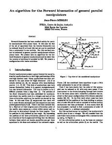
The remainder of this paper is organized as follows. In Section 2, a classification of six-degrees-of-freedom parallel mechanisms based on the number of base and manipulator platform joints as well as combinatorial classes is introduced. In Section 3, we investigate if a closed-form solution for the direct kinematics problem of the mechanism types presented in Section 2 is possible by only measuring the orientations of the linear actuators. In Section 4, for the mechanism types where a closed-form solution of the direct kinematics problem is not possible by only measuring the linear actuators’ orientations, we also include the information about the roll-pitch orientation of the manipulator platform. In Section 5, we discuss the last remaining case where also the information about the manipulator platform’s yaw orientation is included. In order to complete our systematic investigation, in Section 6, we extend our results to threedegrees-of-freedom planar mechanisms. Section 7 discusses some practical considerations regarding the sensor selection and implementation of the proposed algorithms in a realtime control. Finally, in Section 8, our results are summarized and discussed. Throughout the paper, we use the following notation, referring to Figure 1. The body-fixed frame of the base platform is denoted as {1} and the body-fixed frame of the manipulator platform as {2}. The position vector of the 𝑘th joint 𝐽𝑘,𝑖 of platform {𝑖} is denoted as p𝑖𝐽𝑘,𝑖 and the connection vector between the joints 𝐽𝑘,1 and 𝐽𝑘,2 of platforms {1} and {2} as p𝐽𝑘,1 𝐽𝑘,2 with 𝑘 ∈ {1, . . . , 6}. Using inverse kinematics, this vector can be determined from 1

p𝐽𝑘,1 𝐽𝑘,2 = 1 p12 + 1 R2 ⋅ 2 p2𝐽𝑘,2 − 1 p1𝐽𝑘,1

2. Classification of Six-Degrees-of-Freedom Parallel Mechanisms Typically, parallel mechanisms are classified by the number of joints on the base and the manipulator platform. This type of classification, however, is not sufficient for catching all descriptive parameters of a parallel mechanism. For this reason, Faugère and Lazard [9] introduced the notion of a combinatorial class, which is represented by a graph where the edges are the linear actuators and the vertices are the joints (see Figure 2). Here, we use both approaches together to classify parallel mechanisms. 2.1. 𝑛-3 Mechanisms. This group of mechanisms contains 𝑛 base platform joints, with 𝑛 ∈ {3, . . . , 6}, and three manipulator platform joints. Each manipulator platform joint is connected to one, two, or three linear actuators. We can classify this group into two types. In the first type, which shall be referred to as 𝑛-3-I mechanisms, all three manipulator platform joints are connected to exactly two linear actuators. According to [9], this type of mechanisms corresponds to seven combinatorial classes: 3

(2)

In the second type, which shall be referred to as 𝑛3-II mechanisms, the first manipulator platform joint is connected to three linear actuators, the second manipulator platform joint to two linear actuators, and the third manipulator platform joint to one linear actuator. This type of mechanisms corresponds to ten combinatorial classes [9]:

(1)

(3)

with respect to platform {1}. Here, 1 R2 denotes the rotation matrix from frame {2} into frame {1}, and p12 is the vector connecting the origins of platforms {1} and {2}. The roll, pitch, and yaw angles of the manipulator platform shall be denoted as 𝛼, 𝛽, and 𝛾, and the direction, or orientation, of p𝐽𝑘,1 𝐽𝑘,2 is referred to as r𝐽𝑘,1 𝐽𝑘,2 , which has unit length.

2.2. 𝑛-4 Mechanisms. Similar to 𝑛-3 mechanisms, this group of mechanisms can be also classified into two types. The first type, which shall be referred to as 𝑛-4-I mechanisms, is characterized by two manipulator platform joints with each of them connected to two linear actuators and two further manipulator platform joints with each of them connected to

Journal of Robotics

3

one linear actuator. According to [9], this type of mechanisms corresponds to sixteen combinatorial classes: 2 2

2

2

1

2

2

(4)

The second type, which shall be referred to as 𝑛-4-II mechanisms, is characterized by one manipulator platform joint connected to three linear actuators and three further manipulator platform joints with each of them connected to one linear actuator. This type of 𝑛-4 mechanisms corresponds to nine combinatorial classes [9]: 3

three joint positions, on the other hand, define a plane with the normal vector

2

1

p𝐽1,2 𝐽3,2 = 1 p1𝐽3,2 − 1 p1𝐽1,2 .

(10)

1 e𝑧 ⋅ 1 n𝑥1 𝑧1 𝛽 = cos−1 ( 󵄨󵄨11 𝑥 𝑧 󵄨󵄨 ) , 󵄨󵄨 n 1 1 󵄨󵄨 𝑥 𝑦

1

e𝑥1 ⋅ 1 p𝐽1,21 𝐽12,2 𝛾 = cos ( 󵄨󵄨 𝑥 𝑦 󵄨󵄨 ) 󵄨󵄨1 p 1 1 󵄨󵄨 󵄨󵄨 𝐽1,2 𝐽2,2 󵄨󵄨

(11)

−1

2

(6)

2

p𝐽1,2 𝐽2,2 = 1 p1𝐽2,2 − 1 p1𝐽1,2 ,

1 e𝑧 ⋅ 1 n𝑦1 𝑧1 𝛼 = cos−1 ( 󵄨󵄨11 𝑦 𝑧 󵄨󵄨 ) , 󵄨󵄨 n 1 1 󵄨󵄨

2.3. 𝑛-5 Mechanisms. This group of mechanisms is described by twelve combinatorial classes [9]: 2

1

The orientation angles 𝛼, 𝛽, and 𝛾 of the manipulator platform can be then determined from

2

3

(9)

for example, where

(5)

4

n = 1 p𝐽1,2 𝐽2,2 × 1 p𝐽1,2 𝐽3,2 ,

1

𝑥 𝑦

e𝑦1 ⋅ 1 p𝐽1,21 𝐽12,2 = cos ( 󵄨󵄨 𝑥 𝑦 󵄨󵄨 ) , 󵄨󵄨󵄨1 p𝐽1,21 𝐽12,2 󵄨󵄨󵄨 󵄨 󵄨 −1

2.4. 𝑛-6 Mechanisms. This group of mechanisms is associated with six combinatorial classes [9]: 6

4

3

2

2

3

(7)

3. Closed-Form Solution by Only Measuring the Linear Actuators’ Orientations

where 1 e𝑥1 , 1 e𝑦1 , and 1 e𝑧1 are the unit vectors of the base platform in 𝑥1 , 𝑦1 , and 𝑧1 direction, 1 n𝑦1 𝑧1 is the projection of 1 n on the 𝑦1 -𝑧1 plane, 1 n𝑥1 𝑧1 is the projection of 1 n on the 𝑥 𝑦 𝑥1 -𝑧1 plane, and 1 p𝐽1,21 𝐽12,2 is the projection of 1 p𝐽1,2 𝐽2,2 on the 𝑥1 -𝑦1 plane with

In this section, we will investigate if a closed-form solution for the direct kinematics problem of the mechanisms introduced in the previous section is possible by only measuring the orientations of the linear actuators.

= (1 n ⋅ 1 e𝑦1 ) ⋅ 1 e𝑦1 + (1 n ⋅ 1 e𝑧1 ) ⋅ 1 e𝑧1 ,

1 𝑥1 𝑧1

= (1 n ⋅ 1 e𝑥1 ) ⋅ 1 e𝑥1 + (1 n ⋅ 1 e𝑧1 ) ⋅ 1 e𝑧1 ,

n

n

1 𝑥1 𝑦1 p𝐽1,2 𝐽2,2

3.1. 𝑛-3 Mechanisms 3.1.1. Type I. Consider an 𝑛-3-I mechanism where the linear actuators 𝑘 = 1 and 𝑘 = 2 are connected to the manipulator platform joint 𝐽1,2 , the linear actuators 𝑘 = 3 and 𝑘 = 4 to the manipulator platform joint 𝐽2,2 , and the linear actuators 𝑘 = 5 and 𝑘 = 6 to the manipulator platform joint 𝐽3,2 . The positions of these joints, 1 p1𝐽1,2 , 1 p1𝐽2,2 , and 1 p1𝐽3,2 , are defined by the intersection points between the straight lines 𝑔𝑘 through the linear actuators 𝑘 = 1, . . . , 6 with 𝑔𝑘 : 1 p𝑘 = 1 p1𝐽𝑘,1 + 𝜆 𝑘 ⋅ 1 r𝐽𝑘,1 𝐽𝑘,2 ,

1 𝑦1 𝑧1

𝜆 𝑘 ∈ R,

= (1 p𝐽1,2 𝐽2,2 ⋅ 1 e𝑥1 ) ⋅ 1 e𝑥1 + (1 p𝐽1,2 𝐽2,2 ⋅ 1 e𝑦1 ) ⋅ 1 e𝑦1 .

The manipulator platform’s position 1 p12 , on the other hand, can be obtained, for example, from 1

p12 = 1 p1𝐽1,2 − 1 R2 ⋅ 2 p2𝐽1,2 ,

(13)

where 1

(8)

where 1 p𝑘 denote the coordinates of 𝑔𝑘 and 1 r𝐽𝑘,1 𝐽𝑘,2 the measured orientations of the linear actuators. In particular, the intersection point between 𝑔1 and 𝑔2 defines 1 p1𝐽1,2 , the intersection point between 𝑔3 and 𝑔4 defines 1 p1𝐽2,2 , and the intersection point between 𝑔5 and 𝑔6 defines 1 p1𝐽3,2 . These

(12)

R2 =1 R2,𝛼 ⋅ 1 R2,𝛽 ⋅ 1 R2,𝛾

with 1

R2,𝛼

1 0 0 [0 cos 𝛼 sin 𝛼 ] =[ ], [0 − sin 𝛼 cos 𝛼]

(14)

4

Journal of Robotics

1

R2,𝛽

cos 𝛽 0 − sin 𝛽 [ 0 1 0 ] =[ ],

linear actuator 𝑘 = 5 define the two possible positions 1 p1𝐽3,2 of the manipulator platform joint 𝐽3,2 . So, it is not possible to find a unique solution for the direct kinematics problem of 𝑛-4-I mechanisms by only measuring the orientations of the linear actuators.

[ sin 𝛽 0 cos 𝛽 ] 1

R2,𝛾

cos 𝛾 sin 𝛾 0 [− sin 𝛾 cos 𝛾 0] =[ ]. [

0

0

1] (15)

We can see that, by only measuring the orientations of the linear actuators, a unique solution for the direct kinematics problem of 𝑛-3-I mechanisms can be found. 3.1.2. Type II. Now, consider an 𝑛-3-II mechanism where the linear actuators 𝑘 = 1, 𝑘 = 2, and 𝑘 = 3 are connected to the manipulator platform joint 𝐽1,2 , the linear actuators 𝑘 = 4 and 𝑘 = 5 are connected to the manipulator platform joint 𝐽2,2 , and the linear actuator 𝑘 = 6 is connected to the manipulator platform joint 𝐽3,2 . The position 1 p1𝐽1,2 of the joint 𝐽1,2 is defined by the intersection point between two of the straight lines 𝑔1 , 𝑔2 , and 𝑔3 through the linear actuators 𝑘 = 1, 𝑘 = 2, and 𝑘 = 3. Hence, only two orientations of these linear actuators are necessary for defining this position. The position 1 p1𝐽2,2 of the joint 𝐽2,2 , on the other hand, is defined by the intersection point between the straight lines 𝑔4 and 𝑔5 through the linear actuators 𝑘 = 4 and 𝑘 = 5. Both positions define a straight line around which the manipulator platform can virtually rotate. We can now define a sphere, for example, with the center 1 p1𝐽2,2 and the radius |2 p𝐽2,2 𝐽3,2 |. The intersection points between the sphere and the straight line 𝑔6 through the linear actuator 𝑘 = 6 define the two possible positions 1 p1𝐽3,2 of the manipulator platform joint 𝐽3,2 . So, by only measuring the orientations of the linear actuators, it is not possible to find a unique solution for the direct kinematics problem of 𝑛-3-II mechanisms by only measuring the linear actuators’ orientations. 3.2. 𝑛-4 Mechanisms 3.2.1. Type I. Consider an 𝑛-4-I mechanism where the linear actuators 𝑘 = 1 and 𝑘 = 2 are connected to the manipulator platform joint 𝐽1,2 , the linear actuators 𝑘 = 3 and 𝑘 = 4 are connected to the manipulator platform joint 𝐽2,2 , the linear actuator 𝑘 = 5 is connected to the manipulator platform joint 𝐽3,2 , and the linear actuator 𝑘 = 6 is connected to the manipulator platform joint 𝐽4,2 . The position 1 p1𝐽1,2 of the manipulator platform joint 𝐽1,2 is defined by the intersection point between the straight lines 𝑔1 and 𝑔2 through the linear actuators 𝑘 = 1 and 𝑘 = 2, and the position 1 p1𝐽2,2 of the manipulator platform joint 𝐽2,2 is defined by the intersection point between the straight lines 𝑔3 and 𝑔4 through the linear actuators 𝑘 = 3 and 𝑘 = 4. Both positions define a straight line around which the manipulator platform can virtually rotate. We can now define a sphere, for example, with the center 1 p1𝐽2,2 and the radius |2 p𝐽2,2 𝐽3,2 |. The intersection points between the sphere and the straight line 𝑔5 through the

3.2.2. Type II. Now, consider an 𝑛-4-II mechanism where the linear actuators 𝑘 = 1, 𝑘 = 2, and 𝑘 = 3 are connected to the manipulator platform joint 𝐽1,2 , the linear actuator 𝑘 = 4 is connected to the manipulator platform joint 𝐽2,2 , the linear actuator 𝑘 = 5 is connected to the manipulator platform joint 𝐽3,2 , and the linear actuator 𝑘 = 6 is connected to the manipulator platform joint 𝐽4,2 . The position 1 p1𝐽1,2 of the joint 𝐽1,2 is defined by the intersection point between two of the straight lines 𝑔1 , 𝑔2 , and 𝑔3 through the linear actuators 𝑘 = 1, 𝑘 = 2, and 𝑘 = 3. Hence, only two orientations of these linear actuators are necessary for defining this position. We can now define two spheres, for example, the first sphere with the center 1 p1𝐽1,2 and the radius |2 p𝐽1,2 𝐽2,2 | and the second sphere with the same center but with the radius |2 p𝐽1,2 𝐽3,2 |. The intersection points between the first sphere and the straight line 𝑔4 through the linear actuator 𝑘 = 4 define the two possible positions 1 p1𝐽2,2 of the manipulator platform joint 𝐽2,2 , and the intersection points between the second sphere and the straight line 𝑔5 through the linear actuator 𝑘 = 5 define the two possible positions 1 p1𝐽3,2 of the manipulator platform joint 𝐽3,2 . So, in total, we obtain four different possible orientations of the manipulator platform, and it is hence not possible to find a unique solution for the direct kinematics problem of 𝑛-4-II mechanisms by only measuring the linear actuators’ orientations. 3.3. 𝑛-5 Mechanisms. Consider an 𝑛-5 mechanism where the linear actuators 𝑘 = 1 and 𝑘 = 2 are connected to the manipulator platform joint 𝐽1,2 , the linear actuator 𝑘 = 3 is connected to the manipulator platform joint 𝐽2,2 , the linear actuator 𝑘 = 4 is connected to the manipulator platform joint 𝐽3,2 , the linear actuator 𝑘 = 5 is connected to the manipulator platform joint 𝐽4,2 , and the linear actuator 𝑘 = 6 is connected to the manipulator platform joint 𝐽5,2 . The position 1 p1𝐽1,2 of the manipulator platform joint 𝐽1,2 is defined by the intersection point between the straight lines 𝑔1 and 𝑔2 through the linear actuators 𝑘 = 1 and 𝑘 = 2. We can now define two spheres, for example, the first sphere with the center 1 p1𝐽1,2 and the radius |2 p𝐽1,2 𝐽2,2 | and the second sphere with the same center but with the radius |2 p𝐽1,2 𝐽3,2 |. The intersection points between the first sphere and the straight line 𝑔3 through the linear actuator 𝑘 = 3 define the two possible positions 1 p1𝐽2,2 of the manipulator platform joint 𝐽2,2 , and the intersection points between the second sphere and the straight line 𝑔4 through the linear actuator 𝑘 = 4 define the two possible positions 1 p1𝐽3,2 of the manipulator platform joint 𝐽3,2 . So, in total, we obtain four different possible orientations of the manipulator platform, and it is hence not possible to find a unique solution for the direct kinematics problem of 𝑛-5 mechanisms by only measuring the orientations of the linear actuators.

Journal of Robotics

5

3.4. 𝑛-6 Mechanisms. Consider an 𝑛-6 mechanism where the linear actuators 𝑘 ∈ {1, . . . , 6} are connected to the manipulator platform joints 𝐽𝑘,2 . We can now choose three arbitrary linear actuators 𝑙, 𝑝, and 𝑞 with 𝑙, 𝑝, 𝑞 ∈ {1, . . . , 6} and 𝑙 ≠ 𝑝 ≠ 𝑞 and define three straight lines through these linear actuators:

Jp,2

𝑔𝑝 : 1 p𝑝 = 1 p1𝐽𝑝,1 + 𝜆 𝑝 ⋅ 1 r𝐽𝑝,1 𝐽𝑝,2 , 𝜆 𝑝 ∈ R, 1

1

(16)

1

Here, 1 p𝑙 , 1 p𝑝 , and 1 p𝑞 denote the coordinates of 𝑔𝑙 , 𝑔𝑝 , and 𝑔𝑞 , and 1 r𝐽𝑙,1 𝐽𝑙,2 , 1 r𝐽𝑝,1 𝐽𝑝,2 , and 1 r𝐽𝑞,1 𝐽𝑞,2 denote the measured orientations of the linear actuators 𝑘 = 𝑙, 𝑘 = 𝑝, and 𝑘 = 𝑞. Next, we can define two spheres, the first sphere with the center 1 p𝑙 and the radius |2 p𝐽𝑙,2 𝐽𝑝,2 | and the second sphere with the same center but with the radius |2 p𝐽𝑙,2 𝐽𝑞,2 |. In this context, the first sphere has to intersect 𝑔𝑝 and the second sphere 𝑔𝑞 , so that we can write the following two equations: 󵄨󵄨 󵄨󵄨2 2 (1 p𝑝 − 1 p𝑙 ) = 󵄨󵄨󵄨2 p𝐽𝑙,2 𝐽𝑝,2 󵄨󵄨󵄨 , 󵄨 󵄨 󵄨 󵄨 2 󵄨 󵄨2 (1 p𝑞 − 1 p𝑙 ) = 󵄨󵄨󵄨2 p𝐽𝑙,2 𝐽𝑞,2 󵄨󵄨󵄨 . 󵄨 󵄨

(17) (18)

Since we know the angle between 2 p𝐽𝑙,2 𝐽𝑝,2 and 2 p𝐽𝑙,2 𝐽𝑞,2 , we can also write (1 p𝑝 − 1 p𝑙 ) ⋅ (1 p𝑞 − 1 p𝑙 ) = 2 p𝐽𝑙,2 𝐽𝑝,2 ⋅ 2 p𝐽𝑙,2 𝐽𝑞,2 .

(19)

We now have a system of three nonlinear equations, (17), (18), and (19), in three variables (𝜆 𝑙 , 𝜆 𝑝 , and 𝜆 𝑞 ), which, in general, is uniquely not solvable. So, it is not possible to find a unique solution for the direct kinematics problem of 𝑛-6 mechanisms by only measuring the linear actuators’ orientations.

4. Closed-Form Solution by Measuring the Linear Actuators’ Orientations and the Roll-Pitch Orientation of the Manipulator Platform In Section 3, we have shown that, by only measuring the orientations of the linear actuators, it is only possible to find a unique solution for 𝑛-3-I mechanisms. In this section, we will investigate if a closed-form solution for the direct kinematics problem is possible by also including the information about the roll-pitch orientation of the manipulator platform. Consider an 𝑛-𝑚 mechanism with 𝑛 ∈ {3, . . . , 6} and 𝑚 ∈ {3, 4, 5}. Each of these mechanisms contains at least two linear actuators that are connected to one manipulator platform joint 𝐽𝑙,2 . We assume that the measured roll-pitch orientation of the manipulator platform is given by the unit normal vector 1 n. The position 1 p1𝐽𝑙,2 of the manipulator platform joint 𝐽𝑙,2 and the unit normal vector 1 n define a plane, and the desired positions 1 p1𝐽𝑝,2 and 1 p1𝐽𝑞,2 of two other

rJ,2 J,1

p12

rJ,1 J,2

rJ,1 J,2

J p,1

  dq    gq,2 Jq,1

p1J,1

𝑔𝑞 : p𝑞 = p1𝐽𝑞,1 + 𝜆 𝑞 ⋅ r𝐽𝑞,1 𝐽𝑞,2 , 𝜆 𝑞 ∈ R.

Jq,2 gq,1

gp,2

  dp   

x2 p2J,2

rJ,2 J,1

gp,1

𝑔𝑙 : 1 p𝑙 = 1 p1𝐽𝑙,1 + 𝜆 𝑙 ⋅ 1 r𝐽𝑙,1 𝐽𝑙,2 , 𝜆 𝑙 ∈ R,

p2J,2

y2 z2 {2}

y1

{1} z1 x1

p1J,1

Figure 3: Schematic diagram for the algorithm from Section 5.

linear actuators 𝑘 = 𝑝 and 𝑘 = 𝑞, where 𝑝 ≠ 𝑞, are defined by the intersection points between these two linear actuators and the plane. So, by measuring the orientations of four linear actuators as well as the roll-pitch orientation of the manipulator platform, it is possible to obtain a closedform solution for the direct kinematics problem of 𝑛-𝑚 mechanisms with 𝑚 ≠ 6. For 𝑚 = 6, however, our solution strategy fails since 𝑛-6 mechanisms do not have a common connection of at least two linear actuators at the manipulator platform. In this case, the information about the manipulator platform’s orientation leads to the following plane equation: (1 p𝑝 − 1 p𝑙 ) ⋅ 1 n = 0.

(20)

We now have a system of two nonlinear equations, (17) and (20), in two variables (𝜆 𝑙 and 𝜆 𝑝 ), which, in general, is uniquely not solvable. So, by including the information about the roll-pitch orientation of the manipulator platform, it is not possible to find a unique solution for the direct kinematics problem of 𝑛-6 mechanisms.

5. Closed-Form Solution by Measuring the Linear Actuators’ Orientations and the Roll-Pitch-Yaw Orientation of the Manipulator Platform We have seen in Section 4 that the information about the orientations of the linear actuators and the roll-pitch orientation of the manipulator platform is not enough to obtain a closed-form solution for the direct kinematics problem of 𝑛-6 mechanisms. However, we have shown in [29] that, by also including the information about the yaw orientation of the manipulator platform, the direct kinematics problem of 𝑛-6 mechanisms can be uniquely solved. In the following, we will review our solution concept from [29] in the context of a general 𝑛-𝑚 mechanism with 𝑛, 𝑚 ∈ {3, . . . , 6}. Consider the orientations 1 r𝐽𝑝,1 𝐽𝑝,2 and 1 r𝐽𝑞,1 𝐽𝑞,2 of two arbitrarily chosen linear actuators 𝑘 = 𝑝 and 𝑘 = 𝑞, where 𝑝 ≠ 𝑞. These orientations define two pairs of straight lines, 𝑔𝑝,1 and 𝑔𝑝,2 as well as 𝑔𝑞,1 and 𝑔𝑞,2 , with the base vectors 1 p1𝐽𝑝,1

and 1 p2𝐽𝑝,2 as well as 1 p1𝐽𝑞,1 and 1 p2𝐽𝑞,2 (see Figure 3). We can

6

Journal of Robotics

now define two distance vectors between these two pairs of straight lines: 1

1

1

2

1

d𝑝 = r𝐽𝑝,1 𝐽𝑝,2 × ( p12 + R2 ⋅ p2𝐽𝑝,2 − p1𝐽𝑝,1 ) , d𝑞 = 1 r𝐽𝑞,1 𝐽𝑞,2 × (1 p12 + 1 R2 ⋅ 2 p2𝐽𝑞,2 − 1 p1𝐽𝑞,1 ) ,

(21)

where the measured roll, pitch, and yaw orientation of the manipulator platform is summarized in the rotation matrix 1 R2 . Using the identity a × b ≡ ̃a ⋅ b

(22)

with the unique solution −1

−1

x = A c = (A⊤ A) A⊤ c.

(28)

The measurement of the orientations of the other four linear actuators is not necessary here since the positions of the corresponding manipulator platform joints are defined by the manipulator platform’s geometry. Note that a robust way of computing x in this case is by using, for example, the QR decomposition [30].

6. Extension to Planar Mechanisms In this section, we extend our previous findings for spatial mechanisms to three-degrees-of-freedom planar mechanisms. Note that, here, only the roll orientation of the manipulator platform is measured due to the planarity constraint.

where 0 −𝑎𝑧 𝑎𝑦 [ ] ] ̃a = [ [ 𝑎𝑧 0 −𝑎𝑥 ] , [−𝑎𝑦 𝑎𝑥 0 ]

(23)

we can rewrite (21) as

6.1. 𝑛-2 Mechanisms. This group of mechanisms contains 𝑛 base platform joints, with 𝑛 ∈ {2, 3}, and two manipulator platform joints. It can be described by two combinatorial classes:

d𝑝 = 1̃r𝐽𝑝,1 𝐽𝑝,2 ⋅ (1 p12 + 1 R2 ⋅ 2 p2𝐽𝑝,2 − 1 p1𝐽𝑝,1 )

(29)

Now, in order to find the unknown position 1 p12 š x, we have to solve the linear least-squares problem

Now, assume that the linear actuators 𝑘 = 1 and 𝑘 = 2 are connected to the manipulator platform joint 𝐽1,2 , and the linear actuator 𝑘 = 3 is connected to the manipulator platform joint 𝐽2,2 . The position 1 p1𝐽1,2 of the manipulator platform joint 𝐽1,2 is defined by the intersection point between the straight lines 𝑔1 and 𝑔2 through the linear actuators 𝑘 = 1 and 𝑘 = 2. We can now define a circle with the center 1 p1𝐽1,2 and the radius |2 p𝐽1,2 𝐽2,2 |. The intersection points between the circle and the straight line 𝑔3 through the linear actuator 𝑘 = 3 define the two possible positions 1 p1𝐽2,2 of the manipulator platform joint 𝐽2,2 . So, by only measuring the orientations of the linear actuators, it is not possible to find a unique solution for the direct kinematics problem of 𝑛-2 mechanisms. In the next step, we assume that the roll orientation of the manipulator platform is measured in terms of the unit normal vector 1 n. Then, the angle 𝛾 between the manipulator and the base platform can be determined as follows:

‖Ax − c‖2 = min!,

𝛾 = cos−1 (1 e𝑦1 ⋅ 1 n) ,

1 = 1⏟⏟̃r⏟⏟⏟𝐽⏟𝑝,1 ⏟⏟𝐽⏟⏟⏟𝑝,2⏟⏟ ⋅ ⏟⏟⏟p⏟⏟12⏟⏟ šx

šA𝑝

+ 1̃r𝐽𝑝,1 𝐽𝑝,2 ⋅ (1 R2 ⋅ 2 p2𝐽𝑝,2 − 1 p1𝐽𝑝,1 ), ⏟⏟⏟⏟⏟⏟⏟⏟⏟⏟⏟⏟⏟⏟⏟⏟⏟⏟⏟⏟⏟⏟⏟⏟⏟⏟⏟⏟⏟⏟⏟⏟⏟⏟⏟⏟⏟⏟⏟⏟⏟⏟⏟⏟⏟⏟⏟⏟⏟⏟⏟⏟⏟⏟⏟⏟⏟⏟⏟ š−c𝑝

1

1

1

2

1

(24)

d𝑞 = ̃r𝐽𝑞,1 𝐽𝑞,2 ⋅ ( p12 + R2 ⋅ p2𝐽𝑞,2 − p1𝐽𝑞,1 ) ̃r𝐽𝑞,1 𝐽𝑞,2 ⋅ 1⏟⏟⏟p⏟⏟12⏟⏟ = 1⏟⏟⏟⏟⏟⏟⏟⏟⏟⏟⏟ šA𝑞

šx

+ 1̃r𝐽𝑞,1 𝐽𝑞,2 ⋅ (1 R2 ⋅ 2 p2𝐽𝑞,2 − 1 p1𝐽𝑞,1 ). ⏟⏟⏟⏟⏟⏟⏟⏟⏟⏟⏟⏟⏟⏟⏟⏟⏟⏟⏟⏟⏟⏟⏟⏟⏟⏟⏟⏟⏟⏟⏟⏟⏟⏟⏟⏟⏟⏟⏟⏟⏟⏟⏟⏟⏟⏟⏟⏟⏟⏟⏟⏟⏟⏟⏟⏟⏟ š−c𝑞

(25)

where 1 e𝑦1 denotes the unit vector of the base platform in 𝑦1 direction. The manipulator platform’s position 1 p12 , on the other hand, can be obtained, for example, from

where A𝑝 A = [ ] ∈ R6×3 , A𝑞

1

(26)

c𝑝 c = [ ] ∈ R6 . c𝑞

šA

šc

p12 = 1 p1𝐽1,2 − 1 R2 ⋅ 2 p2𝐽1,2 ,

(31)

cos 𝛾 sin 𝛾 R2 = [ ]. − sin 𝛾 cos 𝛾

(32)

where 1

This linear least-squares problem can be reduced to the set of linear equations ⊤ ⊤ ⏟⏟⏟⏟⏟⏟⏟ ⏟⏟⏟⏟⏟ ⏟c⏟ A) x = A (A

(30)

(27)

The measurement of the orientation of the third linear actuator is not necessary here, since the position of the corresponding manipulator platform joint is defined by the manipulator platform’s geometry.

Journal of Robotics

7

6.2. 𝑛-3 Mechanisms. In contrast to 𝑛-2 mechanisms, this group of mechanisms contains three manipulator platform joints. It can be also described by two combinatorial classes: 3

(33)

The measured orientations 1 r𝐽𝑘,1 𝐽𝑘,2 define the straight lines 𝑔𝑘 through the linear actuators 𝑘 = 1, . . . , 3 with 1

1

1

𝑔𝑘 : p𝑘 = p1𝐽𝑘,1 + 𝜆 𝑘 ⋅ r𝐽𝑘,1 𝐽𝑘,2 ,

𝜆 𝑘 ∈ R,

(34)

where 1 p𝑘 denote the coordinates of 𝑔𝑘 . We can now define two circles, for example, the first circle with the center 1 p1 and the radius |2 p𝐽1,2 𝐽2,2 | and the second circle with the same center but with the radius |2 p𝐽1,2 𝐽3,2 |. In this context, the first circle has to intersect 𝑔2 and the second circle 𝑔3 , so that we can write the following two equations: 2 󵄨 󵄨2 (1 p2 − 1 p1 ) = 󵄨󵄨󵄨󵄨2 p𝐽1,2 𝐽2,2 󵄨󵄨󵄨󵄨 , 2 󵄨 󵄨2 (1 p3 − 1 p1 ) = 󵄨󵄨󵄨󵄨2 p𝐽1,2 𝐽3,2 󵄨󵄨󵄨󵄨 .

(35)

Since 2 p𝐽1,2 𝐽2,2 and 2 p𝐽1,2 𝐽3,2 are linearly dependent, we can also write (1 p2 − 1 p1 ) ⋅ (1 p3 − 1 p1 ) = 1.

(36)

We now have a system of three nonlinear equations, (35) and (36), in three variables (𝜆 1 , 𝜆 2 , and 𝜆 3 ), which, in general, is uniquely not solvable. So, it is not possible to find a unique solution for the direct kinematics problem of 𝑛-3 mechanisms by only measuring the orientations of the linear actuators. However, by also including the roll orientation in terms of the rotation matrix (32), we can always apply our general algorithm from Section 5, which always provides a closedform solution of the direct kinematics problem. Note that, in this case, only the measurement of the orientations of two linear actuators is necessary, since the position of the third manipulator platform joint is defined by the manipulator platform’s geometry.

7. Practical Considerations Currently, there are many possible sensors available on the market, spreading from very expensive, precalibrated highprecision sensors to uncalibrated low-cost sensors. In [29], we used the InvenSense MPU-9150 inertial measurement units (IMUs) consisting of an acceleration sensor with three axes, a gyroscope, and a magnetic sensor for determining the closed-form solution for the direct kinematics problem of a general 𝑛-𝑚 mechanism. We obtained the correct solution for selected static poses, but the results showed relatively high mean errors and standard deviations, especially for the yaw orientation of the manipulator platform. This was primarily caused by the noisy and uncalibrated IMUs. The calibration problem, however, can be solved without any additional external equipment by using the

approach from [31]. For example, the acceleration sensor has to be calibrated/corrected in terms of sensor bias, scaling error, and nonorthogonality. In this context, the calibrated measurement data acal can be obtained by the following transformation: acal = TS (au + b) ,

(37)

where au is the uncalibrated acceleration vector and b a constant bias term. The matrix S is a diagonal matrix comprising of scaling factors in each axis, and T is an upper triangular matrix to correct nonorthogonality. Another problem related to calibration is sensor placement. In [29], we mounted the IMUs on the gearboxes of the linear actuators and on top of the manipulator platform. In this context, the alignment of the IMUs regarding the base platform’s coordinate system has to be determined very carefully. One possibility is to use very precise measurement equipment, for example, by using optical or angular sensors to obtain the location of the IMUs on the linear actuators. An alternative way is to determine the sensor alignment by comparing the target orientations with the measured orientations for several predefined poses. In order to achieve a closed-form solution of the direct kinematics problem in hard real-time, the introduced algorithms where the linear actuators’ orientations and, if necessary, the roll-pitch orientation of the manipulator platform are measured are preferable due to the precision of the acceleration sensors. However, the algorithm where also the yaw orientation of the manipulator platform is needed requires the usage of a magnetic sensor, which, in general, is very imprecise. Several information filters, such as Kalman filter or complementary filters, were proposed to obtain the optimal measurement data fusion (see, e.g., [32, 33]). These filters can perform very quickly (between 1.3 and 7 𝜇s [32]), but they do not calculate the correct yaw orientation with the first measurement value. Instead, the calculated yaw orientation only converges towards the correct value within several measurements. As already mentioned above, we tested our approach for the general 𝑛-𝑚 mechanism on several static poses [29]. In the static case, the acceleration sensors measure the constant gravity vector of the earth without any disturbances. Under dynamic conditions, however, in addition to the earth’s gravity field, the acceleration sensors also measure the acceleration of the mechanism itself. Since we can also measure the angular velocities by the available gyroscopes, we are able to compensate these erroneous measurements. In particular, by implementing an information filter for fusing the measurement data of the acceleration sensors, the gyroscopes, and the magnetic sensors of the IMUs, the orientations of the linear actuators can be robustly obtained (see, e.g., [34]). Figure 4 shows the concept for the pose control of parallel mechanisms associated with the introduced algorithms for solving the direct kinematics problem. Here, a target pose ptarget is defined and compared with the actual pose pis leading to the pose deviation Δp. By using inverse kinematics, we can convert Δp into the required length deviation Δl of

8

Journal of Robotics Δp

pＮ；ＬＡ？Ｎ −

Inverse kinematics

Δl

Controller

u

System

y

pＣＭ

Direct kinematics

z

Sensor fusion filter

m

Measurements

Figure 4: Pose control concept for parallel mechanisms using the algorithms from Sections 3–6.

the linear actuators and give it to the controller, for example, a PID controller, as input. The controller then generates the control input u for the system that, in turn, produces the system output y. The measurement vector m that includes the raw data of the acceleration sensors, the gyroscopes, and the magnetic sensors is sent to the sensor fusion filter, for example, a Kalman filter. Here, the orientations of the linear actuators and, if necessary, also the orientation of the manipulator platform are calculated. The filter output z is then used to calculate the actual pose of the manipulator platform pis by using the algorithms introduced in Sections 3–6. In conclusion, the pose of an 𝑛-𝑚 parallel mechanism can be determined by only measuring the linear actuators’ orientations and, if necessary, the orientation of the manipulator platform. The accuracy mainly depends on three things: (1) the precision of the used sensors, (2) their calibration and accurate alignment on the linear actuators and the manipulator platform, and (3) whether we have to measure the yaw orientation or not. For a dynamic pose determination, we have to estimate the linear actuators’ orientations by a suitable sensor fusion.

8. Conclusions We showed that, for 𝑛-3-I mechanisms, it is possible to find a unique solution for the direct kinematics problem by only measuring the orientations of the linear actuators. By also including the information about the roll-pitch orientation of the manipulator platform, it is also possible to uniquely solve the direct kinematics problem for 𝑛-3-II, 𝑛-4, and 𝑛-5 mechanisms. Finally, we demonstrated that the most general case of 𝑛-6 mechanisms also requires the information about the yaw orientation of the manipulator platform. We then extended our approach to planar mechanisms and showed that the direct kinematics problem can be uniquely solved by measuring the linear actuators’ orientations and the roll orientation of the manipulator platform. The results suggest that, in most cases, it is not even necessary to measure the orientations of all six linear actuators. In particular, for 𝑛-3-II, 𝑛-4, and 𝑛-5 mechanisms, additionally to the roll-pitch orientation of the manipulator platform, only the orientations of four linear actuators are needed. By also measuring the yaw orientation of the manipulator platform, the number of required linear actuators’ orientations can be even reduced to two. The case where only the linear actuators’ orientations are measured is advantageous because, then, the sensors can be placed close to the base platform, thus reducing

the wiring effort. Furthermore, only measuring the rollpitch orientation of the manipulator platform provides better results compared to an additional measurement of the yaw orientation [29]. This is especially advantageous, for example, for milling machines, where the yaw degree-of-freedom is not used. Our results enable the design of a low-cost sensor system for parallel mechanisms that provides a unique solution of their direct kinematics problem. This concept is particularly important if no information about the previous states of the parallel mechanism is available, for example, if it is switched on in a certain pose. Furthermore, acceleration or magnetic sensors are significantly smaller than the usual sensors for measuring the linear actuators’ lengths, thus allowing for a reduction of moving equipment as well as extending the workspace. The real-time performance of the proposed sensor concept and the associated closed-form solutions for the direct kinematics problem of parallel mechanisms can be improved by sensor fusion including the information of additional linear actuators’ orientations or sensors.

Conflicts of Interest The authors declare that there are no conflicts of interest regarding the publication of this paper.

Acknowledgments This work was supported by the German Research Foundation (DFG) (Grant SCHL 275/15-1). The publication of this work was also supported by the DFG and Hamburg University of Technology (TUHH) in the funding programme “Open Access Publishing.”

References [1] F. Ronga and T. Vust, “Stewart platforms without computer?” in Proceedings of the International Conference on Real Analytic and Algebraic Geometry, pp. 197–212, Trento, Italy, 1992. [2] K. H. Hunt and E. J. F. Primrose, “Assembly configurations of some in-parallel-actuated manipulators,” Mechanism and Machine Theory, vol. 28, no. 1, pp. 31–42, 1993. [3] D. Lazard, “On the representation of rigid-body motions and its application to generalized platform manipulators,” in Computational Kinematics, G. M. L. Gladwell, J. Angeles, G. Hommel, and P. Kovács, Eds., vol. 28 of Solid Mechanics and Its Applications, pp. 175–181, Springer, Dordrecht, The Netherlands, 1993.

Journal of Robotics [4] B. Mourrain, “The 40 “generic” positions of a parallel robot,” in Proceedings of the International Symposium on Symbolic and Algebraic Computation, pp. 173–182, Kiev, Ukraine, July 1993. [5] M. Raghavan, “Stewart platform of general geometry has 40 configurations,” Journal of Mechanical Design, vol. 115, no. 2, pp. 277–280, 1993. [6] M. Raghavan and B. Roth, “Solving polynomial systems for the kinematic analysis and synthesis of mechanisms and robot manipulators,” Journal of Mechanical Design, vol. 117, pp. 71–79, 1995. [7] M. L. Husty, “An algorithm for solving the direct kinematics of general Stewart-Gough platforms,” Mechanism and Machine Theory, vol. 31, no. 4, pp. 365–379, 1996. [8] P. Dietmaier, “The Stewart-Gough platform of general geometry can have 40 real postures,” in Proceedings of the International Symposium on Advances in Robot Kinematics, pp. 7–16, Strobl, Austria, 1998. [9] J. C. Faugère and D. Lazard, “Combinatorial classes of parallel manipulators,” Mechanism and Machine Theory, vol. 30, no. 6, pp. 765–776, 1995. [10] J.-P. Merlet, Parallel Robots, Springer, Dordrecht, The Netherlands, 2nd edition, 2006. [11] Z. Geng and L. Haynes, “Neural network solution for the forward kinematics problem of a Stewart platform,” in Proceedings of the IEEE International Conference on Robotics and Automation, pp. 2650–2655, Sacramento, CA, USA, April 1991. [12] N. Mimura and Y. Funahashi, “New analytical system applying 6 DOF parallel link manipulator for evaluating motion sensation,” in Proceedings of the IEEE International Conference on Robotics and Automation, pp. 227–233, Nagoya, Japan, May 1995. [13] R. Boudreau and N. Turkkan, “Solving the forward kinematics of parallel manipulators with a genetic algorithm,” Journal of Robotic Systems, vol. 13, no. 2, pp. 111–125, 1996. [14] B. Dasgupta and T. S. Mruthyunjaya, “A constructive predictorcorrector algorithm for the direct position kinematics problem for a general 6-6 Stewart platform,” Mechanism and Machine Theory, vol. 31, no. 6, pp. 799–811, 1996. [15] C. M. Gosselin, “Parallel computational algorithms for the kinematics and dynamics of planar and spatial parallel manipulators,” Journal of Dynamic Systems, Measurement, and Control, vol. 118, no. 1, pp. 22–28, 1996. [16] P. R. McAree and R. W. Daniel, “A fast, robust solution to the Stewart platform forward kinematics,” Journal of Robotic Systems, vol. 13, no. 7, pp. 407–427, 1996. [17] K. Der-Ming, “Direct displacement analysis of a Stewart platform mechanism,” Mechanism and Machine Theory, vol. 34, no. 3, pp. 453–465, 1999. [18] A. K. Dhingra, A. N. Almadi, and D. Kohli, “A GröbnerSylvester hybrid method for closed-form displacement analysis of mechanisms,” Journal of Mechanical Design, vol. 122, no. 4, pp. 431–438, 2000. [19] K. H. Hunt and P. R. McAree, “The octahedral manipulator: geometry and mobility,” The International Journal of Robotics Research, vol. 17, no. 8, pp. 868–885, 1998. ˇ [20] Z. Sika, V. Kocandrle, and V. Stejskal, “An investigation of properties of the forward displacement analysis of the generalized Stewart platform by means of general optimization methods,” Mechanism and Machine Theory, vol. 33, no. 3, pp. 245–253, 1998.

9 [21] R. Stoughton and T. Arai, “Optimal sensor placement for forward kinematics evaluation of a 6-DOF parallel link manipulator,” in Proceedings of the IEEE/RSJ International Workshop on Intelligent Robots and Systems, pp. 785–790, Osaka, Japan, 1991. [22] K. C. Cheok, J. L. Overholt, and R. R. Beck, “Exact methods for determining the kinematics of a Stewart platform using additional displacement sensors,” Journal of Robotic Systems, vol. 10, no. 5, pp. 689–707, 1993. [23] J.-P. Merlet, “Closed-form resolution of the direct kinematics of parallel manipulators using extra sensors data,” in Proceedings of the IEEE International Conference on Robotics and Automation, pp. 200–204, Singapore, Singapore, May 1993. [24] R. Nair and J. H. Maddocks, “On the forward kinematics of parallel manipulators,” The International Journal of Robotics Research, vol. 13, no. 2, pp. 171–188, 1994. [25] L. Baron and J. Angeles, “The direct kinematics of parallel manipulators under joint-sensor redundancy,” IEEE Transactions on Robotics and Automation, vol. 16, no. 1, pp. 12–19, 2000. [26] Y.-J. Chiu and M.-H. Perng, “Forward kinematics of a general fully parallel manipulator with auxiliary sensors,” The International Journal of Robotics Research, vol. 20, no. 5, pp. 401–414, 2001. [27] J. Hesselbach, C. Bier, I. Pietsch et al., “Passive joint-sensor applications for parallel robots,” in Proceedings of the IEEE/RSJ International Conference on Intelligent Robots and Systems, pp. 3507–3512, Sendai, Japan, October 2004. [28] R. Vertechy and V. Parenti Castelli, “Accurate and fast body pose estimation by three point position data,” Mechanism and Machine Theory, vol. 42, no. 9, pp. 1170–1183, 2007. [29] S. Schulz, A. Seibel, D. Schreiber, and J. Schlattmann, “Sensor concept for solving the direct kinematics problem of the Stewart-Gough platform,” in Proceedings of the IEEE/RSJ International Conference on Intelligent Robots and Systems, pp. 1959– 1964, Vancouver, Canada, September 2017. [30] G. H. Golub and C. F. Van Loan, Matrix Computations, vol. 3 of Johns Hopkins Series in the Mathematical Sciences, Johns Hopkins, Baltimore, MD, USA, 1983. [31] U. Qureshi and F. Golnaraghi, “An algorithm for the in-field calibration of a MEMS IMU,” IEEE Sensors Journal, 2017. [32] R. G. Valenti, I. Dryanovski, and J. Xiao, “Keeping a good attitude: a quaternion-based orientation filter for IMUs and MARGs,” Sensors, vol. 15, no. 8, pp. 19302–19330, 2015. [33] S. O. H. Madgwick, A. J. L. Harrison, and R. Vaidyanathan, “Estimation of IMU and MARG orientation using a gradient descent algorithm,” in Proceedings of the IEEE International Conference on Rehabilitation Robotics, pp. 179–185, Zurich, Switzerland, July 2011. [34] X. Yun, M. Lizarraga, E. R. Bachmann, and R. B. McGhee, “An improved quaternion-based Kalman filter for real-time tracking of rigid body orientation,” in Proceedings of the IEEE/RSJ International Conference on Intelligent Robots and Systems, pp. 1074–1079, Las Vegas, NV, USA, October 2003.

International Journal of

Rotating Machinery

Engineering Journal of

Hindawi Publishing Corporation http://www.hindawi.com

Volume 2014

The Scientific World Journal Hindawi Publishing Corporation http://www.hindawi.com

Volume 2014


Distributed Sensor Networks

Journal of

Sensors Hindawi Publishing Corporation http://www.hindawi.com

Volume 2014


Volume 2014


Volume 2014

Journal of

Control Science and Engineering

Advances in

Civil Engineering Hindawi Publishing Corporation http://www.hindawi.com


Volume 2014

Volume 2014

Submit your manuscripts at https://www.hindawi.com Journal of

Journal of

Electrical and Computer Engineering

Robotics Hindawi Publishing Corporation http://www.hindawi.com


Volume 2014

Volume 2014

VLSI Design Advances in OptoElectronics


Navigation and Observation Hindawi Publishing Corporation http://www.hindawi.com

Volume 2014



Chemical Engineering Hindawi Publishing Corporation http://www.hindawi.com

Volume 2014

Volume 2014

Active and Passive Electronic Components

Antennas and Propagation Hindawi Publishing Corporation http://www.hindawi.com

Aerospace Engineering


Volume 2014


Volume 2014

Volume 2014




Modelling & Simulation in Engineering

Volume 2014


Volume 2014

Shock and Vibration Hindawi Publishing Corporation http://www.hindawi.com

Volume 2014

Advances in

Acoustics and Vibration Hindawi Publishing Corporation http://www.hindawi.com

Volume 2014