On the Local Existence for the Characteristic Initial Value Problem in ...

On the Local Existence for the Characteristic Initial Value Problem in General Relativity Jonathan Luk

arXiv:1107.0898v1 [gr-qc] 5 Jul 2011

July 6, 2011 Abstract Given a truncated incoming null cone and a truncated outgoing null cone intersecting at a two sphere S with smooth characteristic initial data, a theorem of Rendall shows that the vacuum Einstein equations can be solved in a small neighborhood of S in the future of S. We show that in fact the vacuum Einstein equations can be solved in a neighborhood in the future of the cones, as long as the constraint equations are initially satisfied on the null cones. The proof is based on energy type estimates and relies heavily on the null structure of the Einstein equations in the double null foliation.

1

Introduction

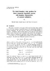
In this paper, we study the characteristic initial value problem of the vacuum Einstein equation. We work in the setting of an outgoing null cone H0 intersecting with an incoming null cone H 0 at a two sphere S0,0 (See Figure 1).

H0

H0

S0,0 Figure 1: Basic Setup It was shown by Rendall [7] that for smooth characteristic initial data prescribed on H0 and H 0 , the Einstein equations can be solved in a neighborhood of the intersecting sphere to the future of the two null cones as shown by the shaded region in the following figure.

H0

H0 S0,0

Figure 2: Region of Existence in Rendall’s Theorem A very natural question which we learned in a talk of Rendall at MSRI in 2009 is whether one has local existence in a neighborhood of the two null cones, instead of only in a neighborhood of the intersecting sphere. 1

One obstruction is that it is not always possible to solve the constraint equations on the initial characteristic hypersurfaces away from the intersecting sphere. Nevertheless, this question can be studied for characteristic initial data set satisfying the constraint equations. We prove that if the constraint equations are satisfied on H0 for 0 ≤ u ≤ I1 and on H 0 for 0 ≤ u ≤ I2 for some I1 , I2 > 0, then there exists ǫ such that the Einstein equations can be solved for {0 ≤ u ≤ I1 } ∩ {0 ≤ u ≤ ǫ} and {0 ≤ u ≤ I2 } ∩ {0 ≤ u ≤ ǫ} as indicated in the following figure. Moreover, ǫ depends only on the size (measured in appropriate norms) of the characteristic initial data.

u

I1

u

I2 ǫ

ǫ

Figure 3: Improved Region of Existence

Theorem 1. Given regular characteristic initial data that satisfy the constraint equations, there exists a regular solution to the Einstein equations (unique in the double null foliation) in a neighborhood to the future of the null cones. Moreover, the size of the neighborhood can be made to depend only on the size of the initial data. A precise formulation of characteristic initial value problem and the theorem, as well as the definition of the notion of regular initial data can be found in the next section. Notice that while we work with smooth characteristic initial data, the size of the neighborhood in the above theorem depends only on the H 5 norm of the metric. Moreover, using a standard approximation procedure, we can construct an H 4 solution to the Einstein equations given H 5 characteristic initial data. An argument to improve the regularity of this theorem is sketched in Section 7.3. Rendall’s original work covers also the case where the initial characteristic data are prescribed on two intersecting null hyperplanes. Our method can also be extended to this case to show that if the constraints are satisfied, the Einstein equations can be solved in a neighborhood to the future of the null hyperplanes. Recently, Choquet-Bruhat, Chrusciel and Martin-Garcia [1] studied the case where the initial characteristic data are prescribed on a cone. They constructed data satisfying the constraints and solved the Einstein equations near the vertex. One reason for studying the characteristic initial value problem is that contrary to the usual Cauchy problem in general relativity, the constraint equations for the characteristic initial value problem are of the type of transport equations. They are therefore much easier to analyze compared to the constraint equations for the Cauchy problem. This can be used to construct special initial data set for which the dynamics can be understood. An important example is the recent monumental work of Christodoulou on the formation of trapped surfaces [2]. While Rendall’s theorem holds for general quasilinear wave equations, our theorem only holds when a special “null structure” is present in the equation. In Section 7.1, we will show that the ideas in this paper can be modified to treat the case of a semilinear wave equation with a null condition in 3 + 1 Minkowski space. In Section 7.2, we will also indicate how a corresponding statement fails for a general semilinear wave equation not satisfying the null condition. This thus shows the importance of the structure of the Einstein’s equations in the double null foliation. We now indicate the main ideas in the proof. We foliate the spacetime with outgoing null hypersurfaces Hu and incoming null hypersurfaces H u such that the characteristic initial value is prescribed on H0 and H 0 . Then define an appropriately normalized null frame {e1 , e2 , e3 , e4 } such that e3 is tangent to H u , e4 is tangent to Hu , and {e1 , e2 } is a frame tangent to the 2-spheres where Hu and H u intersect. Define the Ricci coefficients ψ = g(Deµ eν , eσ ) and the null curvature components Ψ = R(eµ , eν, eσ , eδ ) with respect to this frame. We would like to show that for characteristic initial value of size ∼ 1 satisfying the constraint equations for 0 ≤ u ≤ I (for some I > 0) and u = 0, there is a sufficiently small ǫ such that we can prove 2

estimates for the curvature and Ricci coefficients of the spacetime in the region 0 ≤ u ≤ I and 0 ≤ u ≤ ǫ. This would then allow us to prove that existence of solution in this region. Following the general strategy in [3], [5], [2] etc., we prove the desired estimates in two steps. In the first step, we assume the (L2 ) bounds on the (derivatives of the) curvature component and try to prove estimates for the Ricci coefficients. ∇3 ψ = Ψ + ψψ, ∇4 ψ = Ψ + ψψ. The difficulty is to integrate the nonlinear terms. For the ∇3 equations, we can take advantage of the small ǫ length and show that the Ricci coefficients have norms very close to their initial value. However, there are two components, namely, η and ω, that do not satisfy a ∇3 equation but satisfy only a ∇4 equation. The key observation is that for the ∇4 η equation, all the nonlinear terms are of the form that at least one of the factors can be estimated by a ∇3 equation. In other words, the terms η 2 , ω 2 and ηω do not appear. Since using the ∇3 equations we have already established that the norms for at least one of the factors have norms very close to their initial value, the equation becomes essentially linear. Once η is estimated, we can move to the ∇4 ω equation, for which ω2 does not appear in the nonlinear term and we can therefore integrate and prove estimates for all the Ricci coefficients. The second step is the energy estimates for the curvature components. Neglecting derivatives, these are L2 estimates of the form Z Z Z Ψ2 + Ψ2 ≤ R0 + ψΨ2 . Hu

Hu

Du,u

R If either one of the curvature components Ψ in the error term Du,u ψΨ2 can be controlled on Hu , we can integrate along the u direction to gain a power of ǫ. However, the component α cannot be controlled on Hu but can only be controlled on H u . In order to control the term with α2 , we notice that the Ricci coefficient coupling to it satisfies a ∇3 equation and thus can be controlled by a constant depending only on the initial data. Hence this term can be controlled using the Gronwall inequality. In the next section, we will lay out the basic setup, define the double null foliation and write down the equations in our setting. In section 3, we will prove Rendall’s result [7] in the double null foliation using his reduction of the characteristic initial value problem to the Cauchy problem. In section 4, we prove the basic estimates that are necessary for the estimates for the Ricci coefficients and the curvature components. In section 5, we prove the estimates for the Ricci coefficients and the curvature components. Then in section 6, we show that this allows us to prove our main theorem. We conclude in section 7 with some comparisons with semilinear wave equations in 3 + 1 Minkowski space and some discussions on how regularity can be improved for our main theorem. Acknowledgements. The author thanks his advisor Igor Rodnianski for many enlightening discussions, as well as many helpful comments for improving the manuscript.

2 2.1

Basic Setup Canonical Coordinate System

Our basic setup is depicted in the following diagram.

H0

S0,0 Figure 4: Basic Setup

3

H0

The two hypersurfaces H0 and H 0 are prescribed to be null. The intersection of the two hypersurfaces is a spacelike 2-sphere which we denote as S0,0 . We consider a spacetime in the future of the two null cones. In this spacetime, we consider optical functions u and u satisfying the eikonal equation g µν ∂µ u∂ν u = 0,

g µν ∂µ u∂ν u = 0,

where u = 0 on H0 and u = 0 on H 0 . Let L′µ = −2g µν ∂ν u, Define Define and

L′µ = −2g µν ∂ν u.

2Ω−2 = −g(L′ , L′ ). e3 = ΩL′ , e4 = ΩL′ . L = Ω2 L ′ , L = Ω2 L ′ .

We will denote the level sets of u as Hu and the level sets of u and H u . By virtue of the Eikonal equations, Hu and H u are null hypersurface. We will use the notation Hu (u′ , u′′ ) to denote the part of the hypersurface Hu with u′ ≤ u ≤ u′′ . We will also use H u (u′ , u′′ ) in the obvious way. Notice that the sets defined by fixed values of (u, u) are 2-spheres. We denote such spheres by Su,u . They are intersections of the hypersurfaces [ Su,u′ by Du,u . Hu and H u . We will also denote the region 0≤u′ ≤u,0≤u′ ≤u

We introduce a coordinate system (u, u, θ1 , θ2 ) as follows: On the sphere S0,0 , define a coordinate system 1 2 (θ , θ ) in a coordinate patch U for the sphere. On H0 , we define the coordinate system (u, θ1 , θ2 ) such that ∂ ∂u = L is tangent to the null geodesics that generate H0 . We then define the coordinate system in the full spacetime by letting u and u to be solutions to the Eikonal equations as above and define θ1 , θ2 by L(θA ) = 0.

For each coordinate patch U , a system of coordinates (u, u, θ1 , θ2 ) is thus defined on DU , where DU is defined to be the image of first applying the diffeomorphism generated by L on H 0 , then applying the diffeomorphism generated by L. In these coordinates, we have   ∂ −1 −1 ∂ A ∂ , , e4 = Ω e3 = Ω +b ∂u ∂u ∂θA for some bA such that bA = 0 on H0 . In these coordinates, the metric is g = −2Ω2 (du ⊗ du + du ⊗ du) + γAB (dθA − bA du) ⊗ (dθB − bB du). Here, γAB is the restriction of the spacetime metric to the tangent space of Su,u . We can choose u and u in such a way that Ω = 1 on the initial hypersurfaces H0 and H 0 . From this point onwards, we will make this assumption. This can be thought of as a normalization condition for u and u. When we make the assertion that the spacetime exists up to u ≤ ǫ, we always take into account this normalization of u. We will also use a system of coordinates (u, u, θ1 , θ2 ) which is defined in a similar way as the coordinate system (u, u, θ1 , θ2 ), except for reversing the roles of L and L in the definition. We will use (u, u, θ1 , θ2 ) as a coordinate system near H0 and (u, u, θ1 , θ2 ) as a coordinate system near H 0 .

4

2.2

The Equations

Given a 2-sphere Su,u and (eA )A=1,2 an arbitrary frame tangent to it we define χAB = g(DA e4 , eB ), χAB = g(DA e3 , eB ), 1 1 ηA = − g(D3 eA , e4 ), η A = − g(D4 eA , e3 ) 2 2 1 1 ω = − g(D4 e3 , e4 ), ω = − g(D3 e4 , e3 ), 4 4 1 ζA = g(DA e4 , e3 ) 2 where DA = De(A) . We also introduce the null curvature components,

(1)

αAB = R(eA , e4 , eB , e4 ), αAB = R(eA , e3 , eB , e3 ), 1 1 βA = R(eA , e4 , e3 , e4 ), β A = R(eA , e3 , e3 , e4 ), (2) 2 2 1 1 ρ = R(e4 , e3 , e4 , e3 ), σ = ∗ R(e4 , e3 , e4 , e3 ) 4 4 ∗ Here R denotes the Hodge dual of R. We denote by ∇ the induced covariant derivative operator on Su,u and by ∇3 , ∇4 the projections to Su,u of the covariant derivatives D3 , D4 , see precise definitions in [5]. Moreover, we define φ(1) · φ(2) to be an arbitrary contraction of the tensor product of φ(1) and φ(2) with respect to the metric γ and also (1) (2)

(1) (2)

(1)

(2)

b (2) )AB := φA φB + φB φA − δAB (φ(1) · φ(2) ) for one forms φA , φA , (φ(1) ⊗φ (1)

(2)

(φ(1) ∧ φ(2) )AB := /ǫ AB (γ −1 )CD φAC φBD

(1)

(2)

for symmetric two tensors φAB , φAB .

Define the divergence and curl of totally symmetric tensors to be (div φ)A1 ...Ar := ∇B φBA1 ...Ar ,

(curl φ)A1 ...Ar := /ǫ BC ∇B φCA1 ...Ar ,

where /ǫ is the volume form associated to the metric γ. Define also the trace to be (trφ)A1 ...Ar−1 := (γ −1 )BC φBCA1 ...Ar−1 . Also, denote by

∗

the Hodge dual on Su,u . Observe that, 1 1 ω = − ∇3 (log Ω), ω = − ∇4 (log Ω), 2 2 ηA = ζA + ∇A (log Ω), η A = −ζA + ∇A (log Ω)

(3)

ˆ and χ ˆ be the traceless parts of χ and χ respectively. We separate the trace and traceless part of χ and χ. Let χ Then χ and χ satisfy the following null structure equations: 1 ˆ 2 − 2ωtrχ ∇4 trχ + (trχ)2 = −|χ| 2 ∇4 χ ˆ + trχχ ˆ = −2ω χ ˆ−α 1 ∇3 trχ + (trχ)2 = −2ωtrχ − |ˆ χ |2 2 ˆ = −2ωˆ χ−α ∇3 χ ˆ + trχ χ 1 ∇4 trχ + trχtrχ = 2ωtrχ + 2ρ − χ ˆ·χ ˆ + 2div η + 2|η|2 2 1 1 b + 2ω χ b ˆ − trχχ ˆ + η ⊗η ∇4 χ ˆ + trχˆ χ = ∇⊗η 2 2 1 ∇3 trχ + trχtrχ = 2ωtrχ + 2ρ − χ ˆ·χ ˆ + 2div η + 2|η|2 2 1 1 b + 2ωχ b χ + η ⊗η ∇3 χ ˆ + trχχ ˆ = ∇⊗η ˆ − trχˆ 2 2 5

(4)

The other Ricci coefficients satisfy the following null structure equations: ∇4 η = −χ · (η − η) − β

∇3 η = −χ · (η − η) + β 3 ∇4 ω = 2ωω + |η − η|2 − 4 3 ∇3 ω = 2ωω + |η − η|2 + 4

1 (η − η) · (η + η) − 4 1 (η − η) · (η + η) − 4

1 |η + η|2 + 8 1 |η + η|2 + 8

1 ρ 2 1 ρ 2

(5)

The Ricci coefficients also satisfy the following constraint equations 1 ∇trχ − 2 1 div χ ˆ = ∇trχ + 2

1 ˆ− (η − η) · (χ 2 1 χ− (η − η) · (ˆ 2 1 curl η = −curl η = σ + χ ˆ ˆ ∧χ 2 1 1 K = −ρ + χ ˆ·χ ˆ − trχtrχ 2 4 div χ ˆ=

1 trχ) − β, 2 1 trχ) + β 2

(6)

with K the Gauss curvature of the surfaces S. The null curvature components satisfy the following null Bianchi equations: 1 b + 4ωα − 3(χρ b ∇3 α + trχα = ∇⊗β ˆ +∗ χσ) ˆ + (ζ + 4η)⊗β, 2 ∇4 β + 2trχβ = div α − 2ωβ + ηα, ˆ · β + 3(ηρ +∗ ησ), ∇3 β + trχβ = ∇ρ + 2ωβ +∗ ∇σ + 2χ 1 ∗ 3 ˆ · α − ζ ·∗ β − 2η ·∗ β, ∇4 σ + trχσ = −div ∗ β + χ 2 2 1 ∗ 3 ˆ · α − ζ ·∗ β − 2η ·∗ β, ∇3 σ + trχσ = −div ∗ β + χ 2 2 1 3 ˆ · α + ζ · β + 2η · β, ∇4 ρ + trχρ = div β − χ 2 2 3 1 ˆ · α + ζ · β − 2η · β, ∇3 ρ + trχρ = −div β − χ 2 2 ∇4 β + trχβ = −∇ρ +∗ ∇σ + 2ωβ + 2ˆ χ · β − 3(ηρ −∗ ησ),

(7)

∇3 β + 2trχβ = −div α − 2ωβ + η · α, 1 b + 4ωα − 3(ˆ b ∇4 α + trχα = −∇⊗β χρ −∗ χ ˆ σ) + (ζ − 4η)⊗β 2

In the sequel, we will use capital Latin letters A ∈ {1, 2} for indices on the spheres Su,u and Greek letters µ ∈ {1, 2, 3, 4} for indices in the whole spacetime. It will be useful in the following to use a schematic notation. We will use φ to denote an arbitrary tensorfield. We will denote Ricci coefficients by ψ and null curvature components by Ψ. Unless otherwise stated, ψ will denote an arbitrary Ricci coefficients and Ψ can denote an arbitrary null curvature components. We will simply write ψψ (or ψΨ, etc.) to denote contractions using the metric γ. When we use this notation, the exact way that the tensors are contracted is irrelevant to the argument. Moreover, when using this schematic notation, we will neglect all constant factors.

2.3

Initial Data

On the initial characteristic hypersurface, γ, χ and χ have to satisfy the equations L / L γ = 2χ,

(8)

L / L γ = 2χ,

(9)

6

1 L / L trχ = − (trχ)2 − |χ| ˆ 2γ (10) 2 1 χ|2γ (11) L / L trχ = − (trχ)2 − |ˆ 2 Here L / denotes the restriction of the Lie derivative to T Su,u . This is a notion intrinsic to the null hypersurfaces. Definition 1. By an initial data set, we refer to a quadruple (γ, χ, χ, ζ) such that γ is a positive definite symmetric covariant two tensorfield on S0,0 , χ is a symmetric covariant two tensorfield on S0,u for u ∈ [0, I1 ], χ is a symmetric covariant two tensorfield on Su,0 for u ∈ [0, I2 ], and ζ is a covariant one tensorfield on S0,0 . Definition 2. We say that an initial data set (γ, χ, χ, ζ) is regular if (8), (10) are satisfied on H0 and (9), (11) are satisfied on H 0 , γ is positive definite and that the quantities γ, χ, χ, ζ are C ∞ . On the initial outgoing hypersurface H0 we prescribe the conformal class of the metric γˆAB satisfying in √ coordinates det γˆAB = 1. Similarly, on the initial incoming√hypersurface H 0 we prescribe we prescribe the conformal class of the metric γˆAB satisfying in coordinates det γˆAB = 1. Prescribe also γAB , ζA , trχ and trχ on the two sphere S0,0 . On S0,0 , since γˆAB and γAB are in the same conformal class, γAB = Φ2 γˆAB . By (8), we know that in the canonical coordinates, ∂ γAB = 2χAB = 2χ ˆAB + trχγAB . ∂u On the other hand

∂ ∂Φ ∂ γAB = Φ2 γˆAB + 2Φ γˆAB . ∂u ∂u ∂u

Since we know that (ˆ γ −1 )AB

∂ ∂ γˆAB = log det γˆ = 0, ∂u ∂u

we can identify χ ˆAB =

1 2 ∂ γˆAB , Φ 2 ∂u

and trχ = Notice also that |χ| ˆ 2γ =

2 ∂Φ . Φ ∂u

1 −1 AC −1 BD ∂ ∂ (ˆ γ ) (ˆ γ ) γˆAB γˆCD 4 ∂u ∂u

depends only on γˆ. Thus, (10) can be re-written as ∂ 2 Φ 1 −1 AC −1 BD ∂ ∂ γ ) (ˆ γ ) + (ˆ γˆAB γˆCD = 0. 2 ∂u 8 ∂u ∂u This ordinary differential equation can be solved with the appropriate initial data. Locally, we also know that Φ 6= 0, and thus the solution is regular. In general, we cannot guarantee that the solution to this ODE is regular up to u = 1, but we will only consider data that satisfy this assumption. The equations (9), (11) on H 0 can be solved in a similar fashion.

7

2.4

Integration and Norms

We define the integration on Su,u and Du,u in the natural way: Let U be a coordinate patch on S0,0 and pU be a partition of unity in DU such that pU is supported in DU . Given a function φ, we define the integration by the volume form of the induced metric on Su,u : Z XZ ∞ Z ∞ p φ := φpU det γdθ1 dθ2 . Su,u

−∞

U

−∞

On Du,u , we define integration using the volume form of the spacetime metric Z XZ uZ uZ ∞ Z ∞ p φ := φpU − det gdθ1 dθ2 du′ du Du,u

U

=2

0

XZ

0

u

0

U

Z

−∞

u

0

Z

−∞

∞

−∞

Z

∞

φpU Ω2

−∞

p − det γdθ1 dθ2 du′ du.

There are no canonical volume forms on Hu and H u . We will define integration by Z

φ :=

Hu (0,u)

and

Z

Hu (0,u)

We also write

XZ U

φ :=

0

XZ U

Z

u

∞

−∞

Z

u

0

∞

−∞

Z

Z

Z

p det γdθ1 dθ2 du,

φ2pU Ω

p det γdθ1 dθ2 du.

−∞

Z

∞

−∞

=

Hu

and

φ2pU Ω

∞

=

Z

, Hu (0,I)

Z

.

H u (0,ǫ)

Hu

We define these norms so that the quantities are integrated “near” H0 . We will prove our main theorem near H0 . All the estimates near H 0 follow with identical arguments and one can define the corresponding norms in the obvious manner. With these definitions of integration, we can define the norms that we will use. Let φ be a tensorfield. For 1 ≤ p < ∞, define Z ||φ||pLp (Su,u ) :=

||φ||pLp (Hu ) := ||φ||pLp (H

u)

:=

Z

Z

Su,u

Hu

Hu

< φ, φ >p/2 γ ,

< φ, φ >p/2 γ , < φ, φ >p/2 . γ

Define also the L∞ norm by ||φ||L∞ (Su,u ) := sup < φ, φ >1/2 (θ). γ θ∈Su,u

It is easy to note that all quantities will be the same if we define the norms and integrations instead using the (u, u, θ1 , θ2 ) coordinates.

8

2.5

Statement of the Theorem

We will prove the following theorem: Theorem 2. Given regular initial data on H0 for 0 ≤ u ≤ I. Then there exists ǫ such that a smooth solution to the vacuum Einstein equations exist in the region such that 0 ≤ u ≤ I and 0 ≤ u ≤ ǫ. This solution is unique in the canonical coordinates. Moreover, ǫ can be chosen to depend only on G0 := O0 := R0 :=

sup( sup γAB + det γ + (inf det γ)−1 ) + I,

sup

S⊂H0 , S⊂H 0 U

A,B=1,2

sup

sup

S⊂H0 , S⊂H 0 ψ∈{χ, χ,trχ,ω} ˆ trχ,ω,η,η,ˆ 3 X i=0

+

sup Ψ∈{α,β,ρ,σ,β}

||∇i Ψ||L2 (H0 ) + sup

sup

max{1,

i=0

||∇i ψ||L2 (S) ,

sup Ψ∈{β,ρ,σ,β,α}

max{1,

S⊂H0 , S⊂H 0 Ψ∈{α,β,ρ,σ,β,α}

3 X

2 X i=0

2 X i=0

||∇i Ψ||L2 (H 0 )

||∇i Ψ||L2 (S) ,

1 X i=0

||∇i ψ||L4 (S) ,

!

1 X i=0

||∇i ψ||L∞ (S) },

||∇i Ψ||L4 (S) }.

Moreover, in this spacetime, sup

sup

u,u ψ∈{χ, ˆ trχ,ω,η,η,ˆ χ,trχ,ω}

+

3 X i=0

(sup

sup

u Ψ∈{α,β,ρ,σ,β}

max{

3 X i=0

||∇i ψ||L2 (Su,u ) ,

||∇i Ψ||L2 (Hu ) + sup

2 X i=0

||∇i ψ||L4 (Su,u ) ,

sup

u Ψ∈{β,ρ,σ,β,α}

1 X i=0

||∇i ψ||L∞ (Su,u ) }

||∇i Ψ||L2 (H u ) )

≤C(O0 , R0 , G0 ). With the same argument, we can also prove a similar statement near H 0 . This would then imply our main theorem as stated in the introduction. Remark 1. Notice that the value of G0 does depend on the choice of coordinates.

3

Rendall’s Theorem

In this section, we repeat the proof of Rendall’s Theorem [7]. The main goal of this section is to show that the local existence theorem of Rendall holds for the characteristic initial data prescribed in the double null foliation. Moreover, we show the uniqueness of solutions in the canonical coordinates. The proof in [7] goes in two steps. Firstly, a local existence theorem is proved for general quasilinear wave equations. Then, this theorem is applied to the Einstein equations. Choose the wave coordinates so that Γµ = g νσ Γµνσ = 0. It is well-known that using the wave coordinates, the Einstein equations are equivalent to the so-called reduced Einstein equations ˜ µν = Rµν + gσ(µ Γσ = 0, R ,ν) which can be written as a system of quasilinear wave equations of gµν . It is therefore sufficient to show that the condition for the wave coordinates is satisfied for the solution. In [7], it is shown that given the conformal class of the metrics on the spheres on the initial characteristic hypersurface, one can choose a coordinate system and prescribe the other components of the metric in this coordinate system such that Γµ = 0 on the initial characteristic hypersurfaces. Since Γµ also satisfies a system of quasilinear wave equations, by uniqueness, Γµ is identically zero. The main goal of this section is thus to show that for our prescribed characteristic initial value, we can also introduce a coordinate system so that Γµ = 0 on the initial characteristic hypersurfaces, as in [7]. For completeness, we cite a particular case of Rendall’s Theorem: 9

Theorem 3 (Rendall [7]). Consider a quasilinear wave equation 2 g µν (φ)∂µν φ = F (φ, ∂φ),

(12)

where g and F are smooth in its variables, with smooth initial data φ on two null hypersurfaces H0 and H 0 . (Initial data are prescribed in a way that H0 and H 0 are null.) Suppose that H0 and H 0 intersect in a topological 2-sphere S0,0 . Suppose moreover that all derivatives of φ are continuous up to S0,0 . Then, there exists a small neighborhood of S0,0 in the future of S0,0 such that a unique solution to (12) exists. Using this theorem, we can prove local existence for the Einstein equations in a small neighborhood of S0,0 in the future of S0,0 in the canonical coordinates. Theorem 4. Given a regular initial data set, there exists a small neighborhood to the future of S0,0 such that the Einstein equations can be solved. Proof. We first focus on the outgoing hypersurface H0 . The incoming hypersurface H 0 can be treated analogously. On H0 , consider a coordinate patch for the canonical coordinate system. Rename the coordinates x1 = θ1 , x2 = θ2 , u = x4 . Then let gAB = γAB and g44 = g4A = 0. By (8) and (10), we have gAB,4 = 2χAB , and It is helpful to note that since g4A

1 AB 1 (g gAB,4 ),4 + g AB ,4 gAB,4 = 0. 2 4 = 0 and g44 = 0, we must have g 3A = 0, g 33 = 0, g 34 g34 = 1, and g 33 ,3 = −g 34 g 34 g44,3 .

We would like to prescribe g33 , g34 , g3A on H0 such that the wave coordinate constraints are satisfied and we can solve the reduced Einstein equations. We solve for f3 from the ODE 1 ∂f3 = g AB gAB,4 f3 , (13) 4 ∂x 2 with the initial condition f3 = 1 on S0,0 . Prescribe g34 = −2f3 .

Notice that since f3 ∼ 1, we have g34 ∼ −2 near S0,0 . Thus, near S0,0 , we have g34 6= 0 and g 34 6= 0. In wave coordinates, we would have the condition Γ3 = 0, which, in coordinates, reads

1 AB g gAB,4 g34 . (14) 2 We will for now assume that this is the value of g44,3 . Once we have proved the existence of the spacetime, we will show that this condition is indeed satisfied in the spacetime that we have constructed. Notice that g34 and g44,3 that we prescribe, g44,3 =

R44 =

1 1 1 AB (g gAB,4 ),4 + g AB ,4 gAB,4 − g 34 g AB gAB,4 (2g34,4 − g44,3 ) = 0. 2 4 4 10

We note also that since we have prescribed g34 , we can compute g34,A . On S0,0 , we prescribe g3A by the following procedure. First, we write the prescribed ζA in coordinates. Then we require on S0,0 that g3A,4 − g4A,3 = 4ζA − g34,A .

Moreover, we can write down the wave coordinate condition ΓA = 0, which in coordinates reads ΓA =

1 34 AB 1 g g (gB3,4 + gB4,3 ) + g 34 g A4 g44,3 + ... = 0, 2 2

(15)

where ... represents terms that can be computed from the metric components that we know so far. Now these two conditions give four linearly independent linear equations on g31,4 , g32,4 , g41,3 , g42,3 and hence we can solve for all of these on S0,0 . Now we proceed to prescribe g3A,4 on H0 . We consider the equation R4A = 0 in coordinates, using g44,3 = 12 g AB gAB,4 g34 : 1 1 1 0 = R4A = (g 34 (g3A,4 − g4A,3 )),4 + (g 4B gAB,4 ),4 + g 3B ,3 gAB,4 2 2 2 1 1 CD 34 4B − g gCD,4 (g (g3A.4 − g4A,3 ) + g gAB,4 ) − g BC g 34 gAC,4 g4C,B + ..., 2 2

(16)

where ... denotes terms involving the metric components that we have already prescribed. We note that g 4B is linear in g3C with coefficients that are smooth functions of the metric components that we have already prescribed. We also note that g 3B ,3 is a linear function in g4A,3 in the same sense. If we impose ΓA = 0 and ΓA ,4 = 0, then R4A = (g 34 g3A,4 ),4 + K4A (g3B , g3B,4 , 1), where K4A is a linear function in g3B , g3B,4 , 1 with coefficients being smooth functions of the metric components that we have already prescribed. (16) is thus a second order ordinary differential equation for g3A . We solve this equation with the initial condition on S0,0 g3A = 0 and g3A,4 as found above. Once g3A is retrieved, we also have g4A,3 from the condition (15). As for g44,3 , g4A,3 is not a function that we can prescribe to solve the reduced Einstein equations. We will nevertheless check that g4A,3 is indeed this function in the spacetime that we construct by checking that (15) holds. We now prescribe g33 on H0 . We would impose the condition Γ4 = 0, which in coordinates reads g 34 g33,4 − g AB gAB,3 + g 44 g44,3 + ... = 0,

(17)

where as before, ... denotes terms that we have already prescribed, i.e., terms involving gAB , gA4 , g34 , g3A , g44,3 , g4A,3 and their derivatives along H0 . Notice that g 44 is a linear function in g33 depending on the terms that we have already prescribed.. Now consider the conditions R34 = 0 and RAB = 0. In coordinates, we have 1 1 1 0 = RAB = − (g 34 gAB,4 ),3 − (g 34 gAB,3 ),4 − (g 44 gAB,4 ),4 2 2 2 1 1 34 CD − g g (gAC,3 gBD,4 + gAC,4 gBD,3 ) − g 44 g CD gAC,4 gBD,4 2 2 1 34 1 34 44 34 + g gAB,4 (g g44,3 + 2g g34,3 ) + g gAB,3 (g 34 g34,4 + g CD gCD,4 ) + ... 4 2 Hence, we can write ˜ AB (g33 , g33,4 , gCD,3 , g34,4 , 1), 0 = RAB = − g 34 gAB,34 + K ˜ AB is linear in g33 , g33,4 , gCD,3 , g34,4 , 1 with coefficients being quantities that we have already prewhere K scribed. We now substitute in (17) to get RAB = − g 34 gAB,34 + KAB (g33 , gCD,3 , g34,4 , 1) = 0, 11

(18)

For R34 = 0, we have, in coordinates, 1 1 1 1 0 = R34 = − (g 34 g33,4 ),4 + (g 34 (2g34,4 − g44,3 )),3 + (g AB gAB,4 ),3 − g 44 ,4 g44,3 2 2 2 2 1 AB 1 AC BD 34 44 + g g gBC,4 gAD,3 − g gAB,4 (g g33,4 + g g44,3 ) 4 4 1 34 1 34 44 − g g44,3 (g g33,4 + g g44,3 ) − g 34 g AB g44,3 gAB,3 + ... 4 4 Note that g 44 is linear in g33 and g 34 ,3 is linear in g34,3 and gAB,3 . Suppose we have the condition Γ4 = 0,

Γ3 ,3 = 0.

Then 1 ˜ 34 (g33 , g33,4 , gAB,3 , g34,4 , 1) R34 = − (g 34 g33,4 ),4 + (g 34 g34,4 ),3 + K 2 1 ˜ 34 (g33 , g33,4 , gAB,3 , g34,4 , 1). = (g AB gAB,3 ),4 + (g 34 g34,4 ),3 + K 2 ˜ 34 is a function, linear in g33 , g33,4 , gAB,3 , g34,4 , 1 with coefficients depending on the previously where K prescribed quantities. Now, substituting in (17) and (18), we have R34 = (g 34 g34,4 ),3 + K34 (g33 , gAB,3 , g34,4 , 1) = 0.

(19)

We now have a coupled system of five linear ordinary differential equations (17), (18) and (19) which are first order in g33 , gAB,3 and g34,3 . The initial conditions for the ordinary differential equations are dictated by continuity on H 0 . Thus we want g33 = 0, g34,3 = 0 identically on S0,0 and gAB,3 to be given by the prescribed initial value. Notice that assuming all gµν and gAB,3 , g44,3 , g4A,3 , g34,3 as above, we also have R44,3 = 0. To see this, we use the contracted Bianchi identity ∇µ Gµ4 = 0,

where Gµν = Rµν − 12 gµν R with R being the scalar curvature. First, notice that all the terms in this identity are terms that we have prescribed in the above procedure (i.e., g3A,3 , g33,3 and terms that involve 2 derivatives in the 3 direction do not appear). Then notice that since g 3A = g 33 = 0, R44 = R4A = R34 = RAB = 0 implies R = 0. Now, using R4µ = 0 and R = 0 on H0 , we know that the only potentially non-vanishing term is the 3 derivative of Gµ4 . Thus, we have 1 0 = g 34 ∇3 G44 = g 34 (R44,3 − (g44 R),3 + 2Γµ34 G4µ ) = g 34 R44,3 . 2 The non-vanishing of g 34 in the small neighborhood of S0,0 thus gives R44,3 = 0.

Now we have given gµν on H0 and H 0 . By Rendall’s Theorem 3 on the local existence for quasilinear wave equations, we can solve the reduced Einstein equations. ˜ µ,ν = Rµν + gσ(µ Γσ ,ν) = 0, R which is a system of quasilinear wave equations. We need to show that this solution to the reduced Einstein equations is indeed a solution to the Einstein equations. By the construction of the data, we have prescribed all derivatives of g on S0,0 such that Γµ = 0 and Rµν = 0. We would like to show that in fact Γµ = 0 on H0 and H 0 . As before, we will consider the situation on H0 . H 0 can be treated analogously. Consider the equation ˜ 44 = R44 + g34 Γ3 ,4 = 0. R 12

˜ 44 = 0 is a first order ordinary equation for On H0 , gµν , gµν,A , gµν,4 , gµν,4A , gµν,44 are as prescribed. Hence R 3 g44,3 . Since Γ = 0 and R44 = 0 satisfy the initial conditions and give a solution to the ODE, by uniqueness of solutions, it must be the case that Γ3 = 0 and R44 = 0 on H0 . Thus we have moreover shown that g44,3 = 21 g AB gAB,4 g34 , as indicated before. Now consider ˜ 4A = R4A + 1 g34 Γ3 ,A + 1 g3A Γ3 ,4 + 1 gAB ΓB ,4 = 0. R 2 2 2 The only terms that are not determined by the initial data are g4A,3 , g4A,34 , g44,3 , g44,3A , g44,34 . We know, ˜ 4A = 0 is a system nevertheless that g44,3 , g44,3A , g44,34 can be determined by the condition Γ3 = 0. Hence, R of first order ODEs for g4A,3 . Notice that the highest order term g4A,34 appears in both R4A and 21 g3A Γ3 ,4 . We need to make sure that the coefficient in the highest order term in not degenerate. Indeed the term is 1 1 1 − g 34 g4A,34 + g 34 g4A,34 = − g 34 g4A,34 . 2 4 4 ˜ 4A = 0. Since g4A,3 given by ΓA = 0 We know that g 34 6= 0 near S0,0 and thus we can solve for g4A,3 using R A is a solution, by uniqueness, we must have R4A = 0 and Γ = 0 on H0 . It remains to show that Γ4 = 0. To ˜ AB = R ˜ 34 = R ˜ 44,3 = 0. Using Γ3 = ΓA = 0, do so, we need to consider the equations R ˜ AB = RAB = 0, R ˜ 44 = R ˜ A4 = 0 are The only terms that are not prescribed as initial data and have not been determined by R ˜ AB = − 1 (g 34 gAB,4 ),3 − 1 (g 34 gAB,3 ),4 − 1 g 34 g CD (gAC,3 gBD,4 + gAC,4 gBD,3 ) + 1 g 34 g 34 gAB,4 g34,3 + ... = 0. R 2 2 2 2 We can write

˜ AB = −g 34 gAB,34 + HAB (gCD,3 , g34,3 , 1) = 0, R

(20)

where HAB (gCD,3 , g34,3 , 1) is linear in gCD,3 , g34,3 , 1. Next, using Γ3 = ΓA = 0, we have ˜ 34 = R34 + 1 g34 Γ4 ,4 = 0. R 2 ˜ 44 = Again, we note that terms that are not prescribed as initial data and have not been determined by R ˜ A4 = 0: R ˜ 34 =(g 34 g34,4 ),3 − 1 (g 34 g44,3 ),3 + 1 (g AB gAB,4 ),3 R 2 2 1 34 AB 1 1 AC BD + g g gBC,4 gAD,3 − g g g44,3 gAB,3 + (−g AB gAB,34 + g 44 g44,34 ) + ... = 0. 4 4 4 Thus, we can write

˜ 34 = g 34 g34,34 + H ˜ 34 (gAB,34 , g44,33 , gCD,3 , g34,3 , 1) = 0. R

˜ AB = 0 to replace the term gAB,34 to get We can substitute the equation (20) for R ˜ 34 = g 34 g34,34 + H34 (g44,33 , gCD,3 , g34,3 , 1) = 0. R

(21)

Finally, using Γ3 = ΓA = 0, we also have ˜ 44,3 = R44,3 + g34 Γ3 ,34 = 0. R ˜ 44 = Again, we note that terms that are not prescribed as initial data and have not been determined by R ˜ R34 = 0: ˜ 44,3 = R44,3 + g34 Γ3 ,34 = 0. R ˜ 44,3 = − 1 g 34 g AB (gAB,34 (2g34,4 − g44,3 ) + gAB,4 (2g34,34 − g44,33 )) + 1 g 34 g44,334 ... R 4 4 13

Thus, we can write ˜ 44,3 = 1 g 34 g44,334 + H ˜ 443 (g34,34 , gAB,34 , g44,33 , gCD,3 , g34,3 , 1) = 0, R 4 ˜ is linear in g34,34 , gAB,34 , g44,33 , gCD,3 , g34,3 , 1 with coefficients that have been prescribed as initial where H ˜ 44 = R ˜ 34 = 0. Substituting (20) and (21), we get data or have been determined by R ˜ 44,3 = 1 g 34 g44,334 + H443 (g44,33 , gCD,3 , g34,3 , 1) = 0. R 4

(22)

Therefore, by (20), (21) and (22), we have a coupled system on first order ODEs for gAB,3 , g34,3 , g44,33 . Uniqueness would now demand that Γ4 = Γ3 ,3 = 0, R34 = RAB = R44,3 = 0 on H0 . We have thus established that Γµ = 0 on H0 and, by symmetry, H 0 . It is well-known that Γµ satisfies a system of quasilinear wave equation. Therefore, by the uniqueness part in Theorem 3, Γµ = 0 in the spacetime, whenever it exists. Hence, the solution to the reduced Einstein equations is indeed a solution to the Einstein equations. Thus to conclude the existence result, it remains to show that the solution satisfies the prescribed initial data. To do so, we change coordinates back to our original gauge. Solve for (g −1 )µν ∂µ u∂ν u = 0,

(g −1 )µν ∂µ u∂ν u = 0

with the conditions u = x3 , u = x4 on H0 and H 0 . Now define θ1 , θ2 by ∂θ2 ∂θ1 = = 0. ∂u ∂u We notice that the Jacobian on each point on S0,0 is the identity. Thus in a neighborhood of S0,0 , (θ1 , θ2 , u, u) forms a coordinate system. By virtue of u, u being solutions to the Eikonal equation, it is clear that guu = guu = 0. Clearly, γ and ζ are as prescribed on S0,0 . It remains to show that guu = −2 on H0 and H 0 and that χ and χ are as prescribed on H0 and H 0 respectively. We will first compute guu on H0 . The case for H 0 can be treated analogously. Consider 0=

∂ ∂u ∂2u −1 µν 34 ∂u 34 ((g ) ∂ u∂ u) = g (−g g + ). µ ν 44,3 ∂x3 ∂x3 ∂x3 ∂x3 ∂x4

Using (14), we thus have ∂ ∂u 1 ∂u = g AB gAB,4 3 . ∂x4 ∂x3 2 ∂x ∂u Moreover, we know by continuity and the fact that u = x3 on H 0 that ∂x 3 = 1 on S0,0 . In other words, ∂u satisfies (13) and has the same initial condition as f3 . Thus, ∂x3 = f3 on H0 . Now,

guu = (

∂u −1 ) g34 = −2(f3 )−1 f3 = −2. ∂x3

Finally, we compute that χAB =

1 gAB,4 2

on H0 ,

and χAB =

1 gAB,3 2

on H 0 ,

as desired. Theorem 5. The solution is unique in the canonical coordinates. Proof. Give a solution to the Einstein equations with given initial data, solve the linear wave equation g xµ = 0, 14

∂u ∂x3

with (x1 , x2 , x3 , x4 ) being the original coordinate functions on H0 and H 0 . This gives a change of coordinates in a neighborhood in the future to S0,0 since the Jacobian is the identity matrix on H0 and H 0 . Since the condition for wave coordinates is satisfied, in this new coordinate system we must have Γµ = 0.

(23)

Moreover, since the spacetime is a solution to the Einstein equations, Rµν = 0.

(24)

By the proof of the previous theorem, (23) and (24) together uniquely determine all components of gµν in this new coordinate system. Now since (23) is satisfied, the Einstein equations are equivalent to the reduced Einstein equations. Hence, the metric components satisfy the reduced Einstein equations, which is a quasilinear wave equation. Hence, the metric is uniquely determined.

4

Basic Estimates

In this section, we would like to assume the appropriate boundedness of the Ricci coefficients and would like to obtain three types of basic estimates. First, we would like to control the metric components in the canonical coordinates. Second, we would like to show the equivalence of norms using the control of the metric components. Third, we would like to prove basic estimates for Sobolev embedding, L2 elliptic estimates and estimates for the covariant transport equations. Some estimates that we derive depend on the coordinates we choose. We will derive the estimates near H0 using the coordinate system (u, u, θ1 , θ2 ). The estimates near H 0 will be similar if we use the coordinate system (u, u, θ1 , θ2 ). All estimates will be proved under the following bootstrap assumption: ||(χ, ˆ χ ˆ , trχ, trχ, ζ, ω, ω)||L∞ (Su,u ) ≤ ∆0 ,

(25)

where ∆0 is a large constant to be chosen later. Notice that while the choice of ǫ depends on ∆0 , all the estimates are independent of ∆0 .

4.1

Estimates for Metric Components

We first show that we can control Ω in D with this bootstrap assumption: Proposition 1. For ǫ small enough depending on initial data and ∆0 , there exists C depending only on initial data such that Ω, Ω−1 ≤ C. Proof.

1 1 ∂ −1 1 Ω . ω = − ∇3 log Ω = Ω∇3 Ω−1 = 2 2 2 ∂u Now both ω and Ω are scalars and therefore the L∞ norm is independent of the metric. We can show that Ω−1 is close to the corresponding value of Ω−1 on a sphere that is on the H0 . More precisely, fix u. Then Z u −1 ||Ω − 1||L∞ (Su,u ) ≤ C ||ω||L∞ (Su′ ,u ) du ≤ C∆0 ǫ. 0

This implies both the estimates for Ω and Ω−1 for sufficiently small ǫ. We then show that we can control γ in D with the bootstrap assumption: Proposition 2. Consider a coordinate patch U on S0,0 and define U0,u to be a coordinate patch on S0,u given by the one-parameter diffeomorphism generated by L. DefineSUu,u to be the image of U0,u under the one-parameter diffeomorphism generated by L. Define also DU = 0≤u≤I,0≤u≤ǫ Uu,u . We require det γ to be bounded above and below on U0,u . By the assumption of the regular initial data, each point on S0,u lies 15

in such a U0,u . For ǫ small enough depending on initial data and ∆0 , there exists C and c depending only on initial data such that the following pointwise bounds for γ in DU hold: c ≤ det γ ≤ C. Moreover, in DU ,

|γAB |, |(γ −1 )AB | ≤ C.

Proof. The first variation formula states that L / L γ = 2Ωχ. In coordinates, this means

∂ γAB = 2ΩχAB . ∂u

From this we derive that

∂ log(det γ) = Ωtrχ. ∂u

Define γ0 (u, u, θ1 , θ2 ) = γ(0, u, θ1 , θ2 ). | det γ − det(γ0 )| ≤ C

Z

u

0

|trχ|du′ ≤ C∆0 ǫ.

We thus know that the det γ is bounded above and below. Let Λ be the larger eigenvalue of γ. Clearly, Λ≤C and

X

A,B=1,2

sup γ,

(26)

A,B=1,2

|χAB |2 ≤ CΛ||χ||L∞ (Su,u ) .

Then |γAB − (γ0 )AB | ≤ C

Z

u

0

|χAB |du′ ≤ CΛ∆0 ǫ.

Using the upper bound (26), we thus obtain the upper bound for |γAB |. The upper bound for |(γ −1 )AB | follows from the upper bound for |γAB | and the lower bound for det γ. A consequence of the previous Proposition is an estimate on the surface area of each two sphere Su,u . Proposition 3. sup |Area(Su,u ) − Area(S0,u )| ≤ C∆0 ǫ. u,u

Proof. This follows from the fact that priately small.

√ det γ is pointwise only slightly perturbed if ǫ is chosen to be appro-

With the estimate on the volume form, we can now show that the Lp norms defined with respect to the metric and the Lp norms defined with respect to the coordinate system are equivalent. Proposition 4. Given a covariant tensor φA1 ...Ar on Su,u , we have Z

Su,u

< φ, φ >p/2 γ ∼

r X X ZZ i=1 Ai =1,2

|φA1 ...Ar |p

p det γdθ1 dθ2 .

We can also control b under the bootstrap assumption, thus controlling the full spacetime metric: Proposition 5. In the canonical coordinates, |bA | ≤ C∆0 ǫ. 16

Proof. bA satisfies the equation

∂bA = −4Ω2 ζ A . ∂u

This can be derived from

∂bA ∂ . ∂u ∂θA Now, integrating and using Proposition 4 gives the result. [L, L] = −

4.2

Estimates for Transport Equations

We need to use the null structure equations and the null Bianchi equations to obtain estimates for the Ricci coefficients and the null curvature components respectively. In order to use the equations, we need a way to obtain estimates from the null transport type equations. This can be achieved under the assumption of bounded of trχ and trχ. Proposition 6. Assume sup ||trχ, trχ||L∞ (Su,u ) ≤ 4O0 . u,u

Then there exists ǫ0 = ǫ0 (O0 ) such that for all ǫ ≤ ǫ0 and for every 1 ≤ p < ∞, we have   Z u ′′ ||∇4 φ||Lp (Su,u′′ ) du ||φ||Lp (Su,u ) ≤ C(O0 , I) ||φ||Lp (Su,u′ ) + u′

||φ||Lp (Su,u ) ≤ 2(||φ||Lp (Su′ ,u ) +

Z

u u′

||∇3 φ||Lp (Su′′ ,u ) du′′ ).

Proof. The following identity holds for any scalar f :  Z  Z Z df d f= + Ωtrχf = Ω (e4 (f ) + trχf ) . du Su,u du Su,u Su,u Similarly, we have

d du

Z

f=

Z

Su,u

Su,u


Ω e3 (f ) + trχf .

This can be proved by using a different coordinate system (u, u, θ1 , θ2 ) Hence, taking f = |φ|2γ , we have ||φ||2L2 (Su,u ) = ||φ||2L2 (Su,u′ ) +

Z

||φ||2L2 (Su,u )

Z

=

||φ||2L2 (Su′ ,u )

+

u

u′ u

u′

Z

Z

Su,u′′

  1 2Ω < φ, ∇4 φ >γ + trχ|φ|2γ du′′ 2

  1 2 2Ω < φ, ∇3 φ >γ + trχ|φ|γ du′′ 2 Su′′ ,u

The Proposition is proved using Cauchy-Schwarz on the sphere and the L∞ bounds for Ω and trχ (trχ) which are provided by Proposition 1 and the assumption respectively. For the L4 estimates, take f = |φ|4γ , and we have   Z uZ 1 2 4 4 2 2Ω|φ|γ < φ, ∇4 φ >γ + trχ|φ|γ du′′ ||φ||L4 (Su,u ) = ||φ||L2 (Su,u′ ) + (27) 2 u′ Su,u′′ ||φ||4L4 (Su,u ) = ||φ||2L2 (Su′ ,u ) +

Z

u

u′

Z

Su′′ ,u

2Ω|φ|2γ

  1 < φ, ∇3 φ >γ + trχ|φ|2γ du′′ 2

Again, we conclude using Cauchy-Schwarz on the sphere and the L∞ bounds for Ω and trχ (trχ). The above estimates also hold for p = ∞: 17

Proposition 7. There exists ǫ0 = ǫ0 (O0 ) such that for all ǫ ≤ ǫ0 , we have   Z u ′′ ||∇4 φ||L∞ (Su,u′′ ) du ||φ||L∞ (Su,u ) ≤ C(O0 , I) ||φ||L∞ (Su,u′ ) + u′

||φ||L∞ (Su,u ) ≤ 2(||φ||L∞ (Su′ ,u ) +

Z

u

u′

||∇3 φ||L∞ (Su′′ ,u ) du′′ ).

Proof. This follows simply from integrating along the integral curves of L and L, and the estimate on Ω in Proposition 1. Using this type of estimates we can control the (derivatives of the) Ricci coefficients assuming the appropriate bounds on the (derivatives of the) null curvature components.

4.3

Sobolev Embedding

From the estimate of the metric, we can also show the Sobolev Embedding Theorems on the two spheres Su,u . Proposition 8. There exists ǫ0 = ǫ0 (∆0 , G0 ) such that as long as ǫ ≤ ǫ0 , we have ||φ||L4 (Su,u ) ≤ C(G0 )

1 X i=0

||∇i φ||L2 (Su,u ) .

Proof. We first prove this for scalars. Since we already have a coordinate system, we only need to estimate the volume form. By Proposition 2, however, we know that the volume form q is bounded above and below. Thus, the proposition holds for scalars. Now, for φ being a tensor, let f = |φ|2γ + δ 2 . Then ||f ||L4 (Su,u )




< φ, ∇φ > γ ≤ C ||f ||L2 (Su,u ) + || q ||L2 (Su,u )  ≤ C ||f ||L2 (Su,u ) + ||∇φ||L2 (Su,u ) . |φ|2γ + δ 2

The Proposition can be achieved by sending δ → 0.

Remark 2. The dependence here on the initial data depends on the choice of coordinates on S0,u . It is possible to instead work geometrically by considering the isoperimetric constant. We refer the reader to Section 5.2 in [2] for more on this approach. The exact same proof gives control over the L6 (Su,u ) norm: Proposition 9. There exists ǫ0 = ǫ0 (∆0 , G0 ) such that as long as ǫ ≤ ǫ0 , we have ||φ||L6 (Su,u ) ≤ C(G0 )

1 X i=0

||∇i φ||L2 (Su,u ) .

We can also prove the Sobolev Embedding Theorem for the L∞ norm: Proposition 10. There exists ǫ0 = ǫ0 (∆0 , G0 ) such that as long as ǫ ≤ ǫ0 , we have
||φ||L∞ (Su,u ) ≤ C(G0 ) ||φ||L2 (Su,u ) + ||∇φ||L4 (Su,u ) . As a consequence,

||φ||L∞ (Su,u ) ≤ C(G0 )

2 X i=0

||∇i φ||L2 (Su,u ) .

Proof. The first statement follows from coordinate considerations as in Proposition 8. The second statement follows from applying the first and Proposition 8. 18

Besides the Sobolev Embedding Theorem on the 2-spheres, we also have a co-dimensional 1 trace formula that allows us to control the L4 (S) norm by using the L2 (H) or L2 (H) norm. Proposition 11. Assume sup ||trχ, trχ||L∞ (Su,u ) ≤ 4O0 . u,u

Then 1

1

1

||φ||L4 (Su,u ) ≤ C(O0 , G0 )(||φ||L4 (Su,0 ) + ||φ||L2 2 (Hu ) ||∇4 φ||L4 2 (Hu ) (||φ||L2 (Hu ) + ||∇φ||L2 (Hu ) ) 4 ), 1

1

1

||φ||L4 (Su,u ) ≤ 2(||φ||L4 (S0,u ) + C(G0 )||φ||L2 2 (H ) ||∇3 φ||L4 2 (H ) (||φ||L2 (H u ) + ||∇φ||L2 (H u ) ) 4 ), u

u

Proof. The proof is standard (see for example [5]). We reproduce it here to emphasis that the constant is dependent only on the initial data. We will prove the first statement. The second statement follows analogously. Using (27) and Proposition 9, we have   Z uZ 1 2Ω|φ|2γ < φ, ∇4 φ >γ + trχ|φ|2γ du′′ ||φ||4L4 (Su,u ) =||φ||4L4 (Su,u′ ) + 2 u′ Su,u′′ Z u ≤||φ||4L4 (Su,u′ ) + 4||φ||3L6 (H) ||∇4 φ||L2 (H) + 2O0 ||φ||4L4 (S) du′′ 0 Z u 4 ≤||φ||L4 (Su,u′ ) + 2O0 ||φ||4L4 (Su,u′′ ) du′′ 0

+ C(G0 )||φ||2L4 (Hu ) (||φ||L2 (Hu ) + ||∇φ||L2 (Hu ) )||∇4 φ||L2 (Hu ) .

By Gronwall inequality, we have ||φ||4L4 (Su,u ) ≤C(O0 , G0 )(||φ||4L4 (Su,u′ ) + ||φ||2L2 (Hu ) (||φ||L2 (Hu ) + ||∇φ||L4 (Hu ) )||∇4 φ||L2 (Hu ) ) For the second statement, the proof follows analogously. However, since we are integrating in the u-direction, we can choose ǫ sufficiently small so that the constant is 2.

4.4

Commutation Formulae

We have the following for commutations: Proposition 12. The commutator [∇4 , ∇] acting on an (0, r) S-tensor is given by [∇4 , ∇B ]φA1 ...Ar =[D4 , DB ]φA1 ...Ar + (∇B log Ω)∇4 φA1 ...Ar − (γ −1 )CD χBD ∇C φA1 ...Ar r r X X (γ −1 )CD χBD η A φA1 ...Aˆi C...Ar + − (γ −1 )CD χAi B η D φA1 ...Aˆi C...Ar . i

i=1

i=1

Proof. Since the formula is tensorial, it suffices to consider a basis e1 , e2 on the 2-sphere that is orthonormal. ∇4 ∇B φA1 ...Ar = D4 DB φA1 ...Ar + η B ∇4 φA1 ...Ar −

r X

χBC η A φA1 ...Aˆi C...Ar , i

i=1

where the notation in the last line means replacing the i-th slot by the index C. ∇B ∇4 φA1 ...Ar = DB D4 φA1 ...Ar − ζB ∇4 φA1 ...Ar + χBC ∇C φA1 ...Ar −

r X

χAi B η C φA1 ...Aˆi C...Ar ,

i=1

Subtracting the later equation from the former, and using η = ζ + ∇ log Ω, we can conclude the Proposition. By induction, we get the following schematic formula for multiple commutations: 19

Proposition 13. Suppose ∇4 φ = F0 . Let ∇4 ∇i φ = Fi . Then X X ∇i1 (η + η)i2 ∇i3 F0 + Fi ∼

i1 +i2 +i3 +i4 =i

i1 +i2 +i3 =i

X

+

∇i1 (η + η)i2 ∇i3 χ∇i4 φ

i1

i1 +i2 +i3 +i4 =i−1

∇ (η + η) ∇i3 β∇i4 φ. i2

where by ∇i1 (η+η)i2 we mean the sum of all terms which is a product of i2 factors, each factor being ∇j (η+η) X ∇j1 (η +η)...∇ji2 (η +η). Similarly, for some j and that the sum of all j’s is i1 , i.e., ∇i1 (η +η)i2 = j1 +...+ji2 =i1

suppose ∇3 φ = G0 . Let ∇3 ∇i φ = Gi . Then X ∇i1 (η + η)i2 ∇i3 G0 + Gi ∼ i1 +i2 +i3 =i

X

+

i1

i1 +i2 +i3 +i4 =i−1

X

i1 +i2 +i3 +i4 =i

∇i1 (η + η)i2 ∇i3 χ∇i4 φ

∇ (η + η) ∇i3 β∇i4 φ. i2

Proof. The proof is by induction. We will prove it for the first statement and the second one is analogous. It is obvious that the i = 0 case is true. Assume that the statement is true for i < i0 . Fi0 =[∇4 , ∇]∇i0 −1 φ + ∇Fi0 −1

∼χ∇i0 φ + (η + η)∇4 ∇i0 −1 φ + β∇i0 −1 φ + χ(η + η)∇i0 −1 φ X ∇i1 (η + η)i2 ∇i3 F0 + i1 +i2 +i3 =i0

+

X

i1 +i2 +i3 +i4 =i0

+

X

∇i1 (η + η)i2 ∇i3 χ∇i4 φ

i1 +2i2 +i3 +i4 =i0 −1

∇i1 (η + η)i2 ∇i3 β∇i4 φ.

First notice that the first, third and fourth terms are acceptable. Then plug in the formula for Fi0 −1 = ∇4 ∇i0 −1 φ and get the result. The following further simplified version is useful for our estimates in the next section: Proposition 14. Suppose ∇4 φ = F0 . Let ∇4 ∇i φ = Fi . Then X X ∇i1 ψ i2 ∇i3 F0 + Fi ∼ i1 +i2 +i3 =i

i1 +i2 +i3 +i4 =i

Similarly, suppose ∇3 φ = G0 . Let ∇3 ∇i φ = Gi . Then X ∇i1 ψ i2 ∇i3 G0 + Gi ∼ i1 +i2 +i3 =i

X

i1 +i2 +i3 +i4 =i

∇i1 ψ i2 ∇i3 χ∇i4 φ.

∇i1 ψ i2 ∇i3 χ∇i4 φ.

Proof. We replace β and β using the Codazzi equations, which schematically looks like β = ∇χ + ψχ, β = ∇χ + ψχ.

20

4.5

The General Elliptic Estimates for the Hodge System

We recall the definition of the divergence and curl of a symmetric covariant tensor of arbitrary rank: (div φ)A1 ...Ar = ∇B φBA1 ...Ar , (curl φ)A1 ...Ar = /ǫ BC ∇B φCA1 ...Ar , where /ǫ is the volume form associated to the metric γ. Recall also that the trace is defined to be (trφ)A1 ...Ar−1 = (γ −1 )BC φBCA1 ...Ar−1 . The following elliptic estimate is standard (See for example [3] or [2]): Proposition 15. Let φ be a totally symmetric r + 1 covariant tensorfield on a 2-sphere (S2 , γ) satisfying div φ = f, Then

Z

2

curl φ = g, 2

(|∇φ| + (r + 1)K|φ| ) =

S2

Z

S2

trφ = h.

(|f |2 + |g|2 + rK|h|2 ).

Given a totally symmetric r + 1 covariant tensorfield φ on a 2-sphere (S2 , γ). We can define its totally symmetric derivative by (∇φ)sCA1 ...Ar+1 =

1 (∇C φA1 ...Ar+1 + ∇A1 φCA2 ...Ar+1 + ... + ∇Ai φCA1 ...Aˆi ...Ar+1 + ... + ∇Ar+1 φCA1 ...Ar ). r+1

Then a direct computation would show (see [2], Lemma 7.2) that Proposition 16. Let φ be a totally symmetric r + 1 covariant tensorfield on a 2-sphere (S2 , γ) satisfying div φ = f,

curl φ = g,

trφ = h.

Then φ′ = (∇φ)s satisfies div φ′ = f ′ , where

curl φ′ = g ′ ,

trφ′ = h′ ,

2K 1 ∗ ( ∇g)s + (r + 1)φ − (γ ⊗s h), r+2 r+1 r+1 (∇g)s + (r + 1)K(∗ φ)s , g′ = r+2 r 2 f+ (∇h)s . h′ = r+2 r+2

f ′ = (∇f )s −

Inducting using the previous two Propositions, we can estimate an arbitrary number of derivatives of tensorfields. Proposition 17. Let φ be a totally symmetric r + 1 covariant tensorfield on a 2-sphere (S2 , γ) satisfying div φ = f,

curl φ = g,

trφ = h.

Suppose also that 2 X i=0

Then for i ≤ 3,

||∇i K||L2 (S) ≤ ∞.

i−1 2 X X (||∇j f ||L2 (S) + ||∇j g||L2 (S) + ||∇j h||L2 (S) + ||φ||L2 (S) ) ||∇i K||L2 (S) , G0 ) ||∇i φ||L2 (S) ≤ C( i=0

j=0

21

Proof. In this proof, let φ(n) denote the symmetrized n-th covariant derivative of φ. This is defined inductively: φ′ = (∇φ)s , and φ(n+1) = (φ(n) )′ . Then φ(n) satisfies the following generalized Hodge system: We would also like to show that we can inductively recover all the derivatives from the symmetrized derivatives. It is instructive to first look at the case of 1 derivative. 1 ((r + 1)∇B φA1 ...Ar+1 − ∇A1 φBA2 ...Ar+1 − ∇Ar+1 φBA1 ...Ar ) r+2 1 + (ǫ/ BA1 gA2 ...Ar+1 + /ǫ BA2 gA1 Aˆ2 ...Ar+1 + ... + /ǫ BAr+1 gA2 ...Ar ). r+2

∇B φA1 ...Ar+1 =φ′BA1 ...Ar+1 + =φ′BA1 ...Ar+1

To retrieve higher order derivatives, we claim that the following holds (n)

∇B1 ...∇Bn φA1 ...Ar+1 − φB1 ...Bn A1 ...Ar+1 ∼ f (n−1) + g (n−1) +

X

i+j≤n−1

φ(j) ∇i K

This can be proved inductively. Finally, using Proposition 16, we can derive inductively a div-curl system for φ(n) , which would allow us to conclude using Proposition 15, as long as we can control K. The terms that we need to control are X ||φ(j) ∇i K||L2 (S) ≤ C(||φ||L∞ (S) ||∇2 K||L2 (S) + ||∇φ||L4 (S) ||∇K||L4 (S) + ||∇2 φ||L2 (S) ||K||L2 (S) ). i+j≤2

By Sobolev Embedding in Propositions 8 and 10, we have ||φ||L∞ (S) + ||∇φ||L4 (S) ≤ ||∇2 φ||L2 (S) + ||φ||L2 (S) . We also need to control terms involving K and f, g, h. Using Sobolev Embedding in Propositions 8 and 10, we have 2 X ||∇i K||L2 (S) ||∇2 h||L2 (S) , ||K∇2 h||L2 (S) ≤ ||K||L∞ (S) ||∇2 h||L2 (S) ≤ C(G0 ) i=0

||K∇(f, g)||L2 (S) ≤ ||K||L∞ (S) ||∇(f, g)||L2 (S) ≤ C(G0 ) ||K∇h||L2 (S) ≤ ||K||L∞ (S) ||∇h||L2 (S) ≤ C(G0 ) ||∇Kh||L2 (S) ≤ ||∇K||L4 (S) ||h||L4 (S) ≤ C(G0 )

2 X i=0

2 X i=0

2 X i=0

||∇i K||L2 (S) ||∇(f, g)||L2 (S) ,

||∇i K||L2 (S) ||∇h||L2 (S) ,

||∇i K||L2 (S) (||∇h||L2 (S) + ||∇2 h||L2 (S) ).

In the following, we will only apply the above Proposition for φ a symmetric traceless 2-tensor. For such tensors, it suffices to know its divergence: Proposition 18. Suppose φ is a symmetric traceless 2-tensor satisfying div φ = f. Suppose moreover that 2 X i=0

||∇i K||L2 (S) ≤ ∞. 22

Then, for i ≤ 3, i

||∇ φ||L2 (S)

2 2 X X i (||∇j f ||L2 (S) + ||φ||L2 (S) ). ||∇ K||L2 (S) , G0 ) ≤ C( j=0

i=0

Proof. In view of the previous Proposition, this Proposition follows from curl φ =∗ f. This is a direct computation using that fact that φ is both symmetric and traceless.

5

Estimates

Given C ∞ characteristic initial data, Rendall’s Theorem guarantees a smooth solution in a neighborhood of the intersection of the two null hypersurfaces. We will prove a priori estimates for this solution up to three derivatives of the curvature in L2 . This would then be sufficient to run a standard persistence of regularity argument to show that the solution remains smooth. We can then use a “last slice” argument to show that the solution indeed exist in the full region in which we can prove estimates. We define the initial data norms as follows: Let O0 =

sup

sup

S⊂H0 ,S⊂H 0 ψ∈{χ, ˆ trχ,ω,η,η,ˆ χ,trχ,ω}

R0 =

3 X i=0

+

sup Ψ∈{α,β,ρ,σ,β}

max{1,

3 X i=0

||∇i ψ||L2 (S) ,

||∇i Ψ||L2 (H0 ) +

S⊂H0 ,S⊂H 0 Ψ∈{α,β,ρ,σ,β,α}

i=0

sup Ψ∈{β,ρ,σ,β,α}

max{1,

sup

sup

2 X

2 X i=0

||∇i ψ||L4 (S) ,

||∇i Ψ||L2 (H 0 )

||∇i Ψ||L2 (S) ,

1 X i=0

!

1 X i=0

||∇i ψ||L∞ (S) }.

||∇i Ψ||L4 (S) }.

Notice that the definition of R0 includes terms that are integrated on the hypersurfaces as well as terms that are integrated on 2-spheres. These numbers are fixed by the initial data. They are assumed to be finite. Whenever we would like to refer to a constant that depends only on the initial data, we will use C(O0 , R0 ) (or C(O0 ) etc.). Let 3 X sup sup R= ||∇i Ψ||L2 (Hu ) + sup ||∇i Ψ||L2 (H u ) , sup i=0

u Ψ∈{α,β,ρ,σ,β}

R(S) =

2 X i=0

u Ψ∈{β,ρ,σ,β,α}

sup ||∇i (α, β, ρ, σ, β)||L4 (Su,u ) . u,u

Our main strategy will be as follows: We will prove all the estimates in two steps. In the first step, we will assume the boundedness of R and prove that ǫ can be chosen so that the Ricci coefficients can be controlled by R(S) and the initial data. This can be achieved by considering the null structure equations (4) and (5) as transport equations for the Ricci coefficients, with the null curvature components as source. We then use Propositions 6 and 7 to derive the necessary estimates. As we have mentioned in the introduction, the main observation in deriving these estimates is that either we have a ∇3 equation, for which we have a smallness constant ǫ and can derive the required estimates; or that whenever we have a ∇4 equation, it must be the case that in the nonlinear term Γ · Γ, at least one factor has already been estimated either by a ∇3 equation or by a ∇4 equation that we have considered first. This would allow the ∇4 equations to be considered as essentially linear equations and thus we can derive the necessary estimates by Gronwall inequality. In order to make this strategy work, we need to track which of the terms can be controlled by the size of the initial data alone. The second step is the energy estimates for the curvature components, i.e., the estimates for R. We will derive, by simple integration by parts, the energy estimates that shows that R can be controlled by R0 and 23

nonlinear terms. The nonlinear terms would have the form (neglecting derivatives) ψΨΨ and the energy estimates schematically look like: Z R2 ≤ R0 + ψΨΨ. Du,u

Notice that using the norm R, all curvature components except α can be controlled on Hu . Thus, whenever these components appear in the nonlinear term, we can control them on Hu and integrate in u, thus gaining a smallness constant ǫ. The main difficulty comes from the terms of the form ψα2 . For these terms, we show that ψ can in fact be controlled (in the first step) by the initial data alone. Thus the nonlinear term is essentially linear and we can close the estimates by Gronwall inequality. It is precisely for this reason that we separated the R and the R(S) norms. We would like to show that the R(S) norms can be controlled by initial data alone, i.e., independent of R and thus allow us to control some norms for the Ricci coefficients independent of R. We can then use this to close the energy estimates. We now perform step one of the proof. We will first show the L∞ bounds for the Ricci coefficients. Proposition 19. Assume R < ∞,

R(S) < ∞,

sup ||∇3 η||L2 (Su,u ) < ∞. u,u

Then there exists ǫ0 = ǫ0 (O0 , R0 , sup ||∇3 η||L2 (Su,u ) , R, G0 ) such that for ǫ ≤ ǫ0 , we have u,u

ˆ trχ, χ ˆ , trχ, η, ω||L∞ (Su,u ) ≤ 3O0 , sup ||χ, u,u

sup ||η, ω||L∞ (Su,u ) ≤ C(O0 , R(S), G0 ). u,u

Proof. It suffices to prove the estimates under the bootstrap assumption: ||χ, ˆ trχ, χ ˆ , trχ, η, ω||L∞ (S) ≤ 4O0 .

(28)

This in particular allows us to use Proposition 7. We first estimate the L∞ norm of η. Notice that ω and ηη do not appear in the null structure equation for ∇4 η. Notice also that in this null structure equation, the curvature term does not contain α. Thus, using the Sobolev Embedding in Proposition 10, we can estimate the curvature term using R(S). Thus, Z u ∞ ||η||L (Su,u ) ≤ O0 + CIR(S) + C(O0 )(1 + ||η||L∞ (Su,u′ ) du′ ). 0

By Gronwall’s inequality, ||η||L∞ (Su,u ) ≤ C(O0 , R(S), G0 ) exp(C(O0 )u). Since u ≤ I, we clearly have

sup ||η||L∞ (Su,u ) ≤ C(O0 , R(S), G0 ). u,u

We then move to the estimate for the L∞ norm of ω. Here, the key is to observe that ω 2 does not appear in the equation for ∇4 ω. Moreover, as for the equation for ∇4 η, the curvature term can be controlled by R(S). Thus, Z u

||ω||L∞ (Su,u ) ≤ O0 + CIR(S) + C(O0 , R(S), G0 ) + C(O0 )

0

||ω||L∞ (Su,u′ ) du′ .

As for the estimates for η, we use Gronwall’s inequality to get

||ω||L∞ (Su,u ) ≤ C(O0 , R(S), G0 ) exp(C(O0 )u). As before, since u ≤ I, we clearly have sup ||ω||L∞ (Su,u ) ≤ C(O0 , R(S), G0 ). u,u

24

We now have to close the bootstrap assumptions for χ, ˆ trχ, χ ˆ , trχ, η, ω. We have ∇3 (χ, ˆ trχ) = Ψ + ∇η + ψψ, and ∇3 (ˆ χ, trχ, η, ω) = Ψ + ψψ. Using these it follows from Proposition 6 that ||χ, ˆ trχ||L∞ (S) ≤ 2O0 + Cǫ sup ||∇3 η||L2 (Su,u ) + ǫC(O0 , R, G0 ). u,u

1

||ˆ χ, trχ, η, ω||L∞ (S) ≤ 2O0 + Cǫ 2 R + ǫC(O0 , R, G0 ). By choosing ǫ sufficiently small depending on O0 , R(S), sup ||∇3 η||L2 (Su,u ) , I, we have u,u

ˆ trχ, χ ˆ , trχ, η, ω)||L∞ (Su,u ) ≤ 3O0 , sup ||(χ, u,u

hence improving the bootstrap assumption (28). We will estimate the L4 norms using a similar strategy. Proposition 20. With the same assumptions as in the last proposition, we have some ǫ0 = ǫ0 (O0 , R(S), sup ||∇3 η||L2 (Su,u ) , R, G0 ) u,u

such that for ǫ ≤ ǫ0 , we have

||∇(χ, ˆ trχ, χ ˆ , trχ, η, ω)||L4 (S) ≤ 3O0 , ||∇(η, ω)||L4 (S) ≤ C(O0 , R(S), G0 ).

Proof. We introduce the bootstrap assumptions: ||∇(χ, ˆ trχ, χ ˆ , trχ, η, ω)||L4 (S) ≤ 4O0 .

(29)

In order to estimate the L4 norm of the Ricci coefficient, we will use Proposition 6. It is applicable since the previous Proposition implies the necessary bounds on ||trχ, trχ||L∞ (S) . We first estimate the L4 norm of ∇η. Notice that ∇ω, (∇η)2 do not appear in the null structure equations. The term η∇η appears, but we can estimate it by ||η∇η||L4 (Su,u ) ≤ ||η||L∞ (Su,u ) ||∇η||L4 (Su,u ) and use the estimate for ||η||L∞ (Su,u ) from the previous Proposition. Moreover, notice that α does not appear in the equation and by Sobolev Embedding in Proposition 8, we can control the curvature term by R(S). Putting all these observations together and using Proposition 6 and 19 and (29), we have Z u ||∇η||L4 (Su,u′ ) du′ . ||∇η||L4 (Su,u ) ≤ C(O0 , R(S), G0 ) + C(O0 , R(S), G0 ) 0

By Gronwall’s inequality, ||∇η||L4 (Su,u ) ≤ C(O0 , R(S), G0 ) exp(C(O0 , R(S), G0 )u). Therefore, ||∇η||L4 (Su,u ) ≤ C(O0 , R(S), G0 ).

25

We then move to the estimate for the L4 norm of ∇ω. Here, the key is to observe that (∇ω)2 does not appear in the equation for ∇4 ∇ω and that α does not appear as the curvature term. Using Proposition 6 and 19 and (29), we have, Z u ||∇ω||L4 (Su,u ) ≤ C(O0 , R(S), G0 ) + C(O0 , R(S), G0 ) ||∇ω||L4 (Su,u′ ) du′ . 0

As for the estimates for ∇η, we use Gronwall’s inequality to get ||∇ω||L4 (Su,u ) ≤ C(O0 , R(S), G0 ) exp(C(O0 , R(S), G0 )u). Therefore, ||∇ω||L4 (Su,u ) ≤ C(O0 , R(S), G0 ). Moreover, as in the proof of Proposition 19, ||∇(χ, ˆ trχ, χ ˆ , trχ, η, ω)||L4 (Su,u ) 1

ˆ trχ, χ ˆ , trχ, η, ω)||L4 (Su,u′ ) . ≤2O0 + C(ǫ 2 R + ǫ sup ||∇3 η||L2 (Su,u ) ) + ǫC(O0 , R(S), G0 ) sup ||∇(χ, u,u

u′ ∈[0,u]

Hence, by choosing ǫ sufficiently small depending on O0 , R(S), sup ||∇3 η||L2 (Su,u ) , R, I, we have u,u

ˆ trχ, χ ˆ , trχ, η, ω)||L4 (Su,u ) ≤ 3O0 , sup ||∇(χ, u,u

which improves the bootstrap assumption and gives the desired estimates. We now move on to the L2 norm of the Ricci coefficients: Proposition 21. With the same assumptions as in the Proposition 19, we have some ǫ0 = ǫ0 (O0 , R(S), sup ||∇3 η||L2 (Su,u ) , R, G0 ) u,u

such that for ǫ ≤ ǫ0 , we have ˆ trχ, χ ˆ , trχ, η, ω)||L2 (Su,u ) ≤ 3O0 , sup ||∇2 (χ, u,u

sup ||∇2 (η, ω)||L2 (Su,u ) ≤ C(O0 , R(S), G0 ) u,u

Proof. We make the bootstrap assumption: ˆ trχ, χ ˆ , trχ, η, ω)||L2 (Su,u ) ≤ 4O0 . sup ||∇(χ, u,u

As before, we first estimate ∇2 η and ∇2 ω. Using the L∞ bounds for ψ and L4 bounds for ∇ψ, we have Z u 2 ||∇ η||L2 (Su,u ) ≤ C(O0 , R(S), G0 ) + C(O0 , R(S), G0 ) ||∇2 η||L2 (Su,u′ ) du′ . 0

By Gronwall’s inequality, ||∇2 η||L2 (Su,u ) ≤ C(O0 , R(S), G0 ). We then move to the estimate for the L∞ norm of ω. Here, the key is to observe that ω2 and ηω do not appear in the equation for ∇4 ω. Z u ||∇2 ω||L2 (Su,u′ ) du′ . ||∇2 ω||L2 (Su,u ) ≤ C(O0 , R(S), G0 ) + C(O0 , R(S), G0 ) 0

26

As for the estimates for ∇η, we use Gronwall’s inequality to get ||∇2 ω||L2 (Su,u ) ≤ C(O0 , R(S), G0 ). Moreover, 1

ˆ trχ, χ ˆ , trχ, η, ω)||L2 (Su,u′ ) . ||∇(χ, ˆ trχ, χ ˆ , trχ, η, ω)||L2 (Su,u ) ≤ 2O0 + Cǫ 2 R + ǫC(O0 , R(S), G0 ) sup ||∇(χ, u′ ∈[0,u]

Hence, by choosing ǫ sufficiently small depending on O0 , R(S), sup ||∇3 η||L2 (Su,u ) , R, I, we have u,u

||∇(χ, ˆ trχ, χ ˆ , trχ, η, ω)||L2 (S) ≤ 3O0 , which improves the bootstrap assumption and gives the desired estimates. We have now proved that the estimates for the Ricci coefficients up to two derivatives in L2 (S) can be estimated by a constant depending only on the initial data and R(S). This is enough for us to show that the R(S) norms can be controlled by the initial data alone. This in turn implies that the Ricci coefficients can be controlled by initial data alone. Proposition 22. Assume R < ∞. Then there exists ǫ0 = ǫ0 (O0 , R0 , R) such that for ǫ ≤ ǫ0 , we have R(S) ≤ C(R0 ). Proof. We first prove the weaker statement 2 X i=0

||∇i (α, β, ρ, σ, β)||L2 (Su,u ) ≤ C(R0 ).

This can be achieved by considering the ∇3 null Bianchi equations as transport equations and estimate using Proposition 6. 2 X i=0

||∇i (α, β, ρ, σ, β)||L2 (Su,u ) X

1

≤2R0 + ǫ 2

3 X

Ψ∈{β,ρ,σ,β,α} i=0

||∇i Ψ||L2 (H u ) +

X

X

i1 +i2 +i3 +i4 ≤2 Ψ∈{α,β,ρ,σ,β,α}

||∇i1 ψ i2 ∇i3 ψ∇i4 Ψ||L1u L2 (S)

By Proposition 21, sup u,u

Therefore, X

i1 +i2 +i3 +i4 ≤2

2 X i=0

||∇i ψ||L2 (Su,u ) ≤ C(O0 , R(S), G0 ).

1

||∇i1 ψ i2 ∇i3 ψ∇i4 Ψ||L1u L2 (S) ≤ ǫ 2 C(O0 , R(S), G0 )R+C(O0 , R(S), G0 )

2 Z X i=0

u 0

||∇i α||L2 (Su′ ,u ) du′ .

Hence, by choosing ǫ sufficiently small, we have 2 X i=0

||∇i (α, β, ρ, σ, β)||L2 (Su,u ) ≤ 3R0 + C(O0 , R(S), G0 )

27

2 Z X i=0

0

u

||∇i α||L2 (Su′ ,u ) du′ .

By Gronwall’s inequality and that u ≤ ǫ, we thus have 2 X i=0

||∇i (α, β, ρ, σ, β)||L2 (Su,u ) ≤ 4R0 .

We now estimate the L4 (S) norms of ∇i (α, β, ρ, σ, β) using the codimension 1 trace formula in Proposition 11. Take φ = ∇i (α, β, ρ, σ, β) for i ≤ 2 and substitute into 1

1

1

||φ||L4 (Su,u ) ≤ 2(||φ||L4 (S0,u ) + C(G0 )||φ||L2 2 (H ) ||∇3 φ||L4 2 (H ) (||φ||L2 (H u ) + ||∇φ||L2 (H u ) ) 4 ). u

u

By definition of the R and R(S) norms, we have 2 X i=0

||∇(∇i (α, β, ρ, σ, β))||L2 (H u ) ≤ C(O0 , R(S), R, G0 ).

and, using the null Bianchi equations, we also have 2 X i=0

≤

||∇3 (∇i (α, β, ρ, σ, β))||L2 (H u )

3 X

X

i=0 Ψ∈{β,ρ,σ,β,α}

||∇i Ψ||L2 (H u ) +

X

X

i1 +i2 +i3 +i4 ≤2 Ψ∈{α,β,ρ,σ,β,α}

||∇i1 ψ i2 ∇i3 ψ∇i4 Ψ||L2 (H u ) .

The first term is clearly ≤ CR. Using Sobolev Embedding in Propositions 8 and 10, as well as the estimates for the Ricci coefficients from Propositions 19, 20 and 21, we have X

X

i1 +i2 +i3 +i4 ≤2 Ψ∈{α,β,ρ,σ,β,α}

||∇i1 ψ i2 ∇i3 ψ∇i4 Ψ||L2 (H u ) ≤ C(O0 , R(S), G0 )

2 X i=0

||∇i Ψ||L2 (H u ) .

Notice that all components except α can be controlled in L2 (H u ), we have 2 X i=0

1

||∇3 (∇i (α, β, ρ, σ, β))||L2 (H u ) ≤ CR + C(O0 , R(S), R0 , G0 )(R + ǫ 2 sup ||α||L2 (Su,u ) . u,u

The smallness parameter that we need for the estimates comes in through the L2 (S) estimates that we have just derived: 2 X i=0

1

||∇i (α, β, ρ, σ, β)||L2 (H u ) ≤ ǫ 2 sup u,u

2 X i=0

1

||∇i (α, β, ρ, σ, β)||L2 (Su,u ) ≤ ǫ 2 C(O0 , R(S), R, G0 ).

Therefore, 2 X i=0

2 X 1 ||∇i (α, β, ρ, σ, β)||L4 (Su,u ) ≤ 2( ||∇i (α, β, ρ, σ, β)||L4 (S0,u ) + ǫ 4 C(O0 , R(S), R, G0 )). i=0

The necessary estimate follows by choosing ǫ sufficiently small. This implies that in Propositions 19, 20 and 21,the bounds can be in terms of initial data alone. In other words, Proposition 23. Assume R < ∞,

sup ||∇3 η||L2 (Su,u ) < ∞. u,u

28

Then there exists ǫ0 = ǫ0 (O0 , R(S), sup ||∇3 η||L2 (Su,u ) , R, G0 ) such that for ǫ ≤ ǫ0 , we have u,u

||ψ||L∞ (Su,u ) ≤ C(O0 , R0 , G0 ), 1 X

||∇i ψ||L4 (Su,u ) ≤ C(O0 , R0 , G0 ),

i=0

2 X

||∇i ψ||L2 (Su,u ) ≤ C(O0 , R0 , G0 ).

i=0

These estimates allow us also to derive estimates for the Gauss curvature K on the spheres. Proposition 24. Assume R < ∞. Then there exists ǫ0 = ǫ0 (O0 , R0 , R) such that for ǫ ≤ ǫ0 , we have 2 X i=0

||∇i K||L2 (S) ≤ C(O0 , R0 , G0 ).

Proof. We estimate ∇i K in L4 (S) using the Gauss equation 1 1 K = −ρ + χ ˆ·χ ˆ − trχ · trχ. 2 4 Proposition 22, 3 and Holder’s inequality give 2 X i=0

||∇i ρ||L2 (Su,u ) ≤ C(O0 , R0 , G0 ).

The R(S) estimates in Proposition 22, together with Proposition 21, give 2 X i=0

||∇i (trχ, trχ, χ, ˆ χ ˆ )||L2 (Su,u ) ≤ C(O0 , R0 , G0 ).

The R(S) estimates in Proposition 22, together with Proposition 19, imply 1 X i=0

||∇i ψ||L∞ (Su,u ) ≤ C(O0 , R0 , G0 ).

Putting all these together, we get the conclusion of the Proposition. In order to close the energy estimates, we will need L2 estimates of up to 3 derivatives of the Ricci coefficients. The proof of this required L2 estimate is analogous to that in the previous Proposition, except for ∇3 χ, ˆ ∇3 trχ since for that we will need estimates for ∇4 η. This can in principle be achievable by elliptic estimates. However, we will take another route. We will use instead the ∇4 equation for ∇3 trχ and retrieve the estimates for ∇3 χ ˆ through elliptic estimates. At this level of derivatives, the ∇4 equation looks linear in the highest order term. Therefore, we can still achieve estimates that depends only on the initial data. Notice that, however, we cannot control ∇3 (η, ω) by the initial data and R(S) alone, but need to use R as well. Proposition 25. Assume R < ∞. Then there exists ǫ0 = ǫ0 (O0 , R0 , R, G0 ) 29

such that for ǫ ≤ ǫ0 , we have

sup ||∇3 (ˆ χ, trχ, η, ω)||L2 (Su,u ) ≤ 3O0 , u,u

sup ||∇3 (χ, ˆ trχ)||L2 (Su,u ) ≤ C(O0 , R0 , G0 ), u,u

sup ||∇3 (η, ω)||L2 (Su,u ) ≤ C(O0 , R0 , R, G0 ). u,u

Proof. We introduce the bootstrap assumptions: χ, trχ, η, ω)||L2 (Su,u ) ≤ 4O0 , sup ||∇3 (ˆ u,u

sup ||∇3 η||L2 (Su,u ) ≤ ∆, u,u

where ∆ is large and will be chosen later. We take ǫ∆ ≪ 1. We first estimate ∇3 χ ˆ and ∇3 trχ. Unlike in the previous Propositions, we no longer use the ∇3 equations because of the loss in derivative. Instead we will use the ∇4 transport equation for ∇3 trχ together with the Codazzi equation. Commute the equation for ∇4 trχ with ∇3 , we get X X ∇i1 ψ i2 ∇i3 χ∇i4 trχ ˆ2 ) + ∇i1 ψ i2 ∇i3 ((trχ)2 + χ ∇4 (∇3 trχ) = i1 +i2 +i3 +i4 =3

i1 +i2 +i3 =3

Notice that in this equation, the only ∇3 derivatives occur in the terms ∇3 trχ and ∇3 χ. ˆ Hence in order to estimate these terms, we do not need to use the bounds in bootstrap assumption. (We do, however, still need to use the bootstrap assumption in order to apply the previous Propositions.) Now, the right hand side of the equation consists of three kinds of terms. In the first situation, we have ∇3 trχ or ∇3 χ. ˆ Then all the other terms do not have derivatives and can be estimated in L∞ (Su,u ) by C(O0 , R0 , G0 ) by Proposition 23: ||ψ∇3 χ||L2 (Su,u′ ) ≤ ||ψ||L∞ (Su,u′ ) )||∇3 (trχ, χ)|| ˆ L2 (Su,u′ ) ≤ C(O0 , R0 , G0 )||∇3 (χ, ˆ trχ)||L2 (Su,u′ ) . In the second situation, the term has one factor of ∇2 ψ. Then the other factors have at most one derivative. Then, we can estimate using Proposition 23: ||∇ψ∇2 ψ + ψψ∇2 ψ||L2 (Su,u′ ) ≤ (||∇ψ||L∞ (Su,u′ ) + ||ψ||2L∞ (Su,u′ ) )||∇2 ψ||L2 (Su,u′ ) ≤ C(O0 , R0 , G0 ). For the third kind of terms, all factors can be controlled in L∞ : ||ψ(∇ψ)2 + ψ 3 ∇ψ + ψ 5 ||L2 (Su,u′ ) ≤ C(O0 , R0 , G0 ). Using Proposition 6, we can estimate ∇3 trχ by ||∇3 trχ||L2 (Su,u ) ≤ C(O0 , R0 , G0 ) + C(O0 , R0 , G0 )

Z

u 0

||∇3 (χ, ˆ trχ)||L2 (Su,u′ ) du′ .

By Gronwall’s inequality, we have ||∇3 trχ||L2 (Su,u ) ≤ C(O0 , R0 , G0 ) + C(O0 , R0 , G0 )

Z

0

u

||∇3 χ|| ˆ L2 (Su,u′ ) du′ .

Using Proposition 18 for the Codazzi equation div χ ˆ=

1 1 1 ˆ − trχ) − β, ∇trχ − (η − η) · (χ 2 2 2

we have ||∇3 χ|| ˆ L2 (Su,u ) ≤ C||∇3 trχ||L2 (Su,u ) + C||∇2 β||L2 (Su,u ) + C(O0 , R0 , G0 ). Notice that we need the estimates for K to apply Proposition 18. This is provided by Proposition 24. Plugging in the estimate for ||∇3 trχ||L2 (Su,u ) as well as the estimate for β in Proposition 22, we have Z u ˆ L2 (Su,u′ ) du′ ). ||∇3 χ|| ||∇3 χ|| ˆ L2 (Su,u ) ≤ C(O0 , R0 , G0 )(1 + 0

30

Thus, by Gronwall’s inequality, we have ||∇3 χ|| ˆ L2 (Su,u ) ≤ C(O0 , R0 , G0 ). We now estimate the L2 norms of ∇3 η and ∇3 ω. These are analogous to the proof of the previous Proposition, except that now the estimates depend also on R. This can be improved using elliptic estimates, but since such improvements will not be used later, we will be content with the dependence on R. Using the L∞ bounds for ψ and ∇ψ and the L4 bounds for ∇2 ψ, we have Z u ||∇3 η||L2 (Su,u′ ) du′ . ||∇3 η||L2 (Su,u ) ≤ C(O0 , R0 , R, G0 ) + C(O0 , R(S), G0 ) 0

By Gronwall’s inequality, ||∇3 η||L2 (Su,u ) ≤ C(O0 , R0 , R, G0 ). Notice that the right hand side does not depend on ∆. We can therefore choose ∆ large so that this estimate improves the bootstrap assumption. We then move to the estimate for the L2 norm of ∇3 ω. Z u 3 ||∇3 ω||L2 (Su,u′ ) du′ . ||∇ ω||L2 (Su,u ) ≤ C(O0 , R0 , R, G0 ) + C(O0 , R0 , G0 ) 0

As for the estimates for ∇η, we use Gronwall’s inequality to get ||∇3 ω||L2 (Su,u ) ≤ C(O0 , R0 , R, G0 ). We now move to close the rest of the bootstrap assumptions: 1

||∇3 (ˆ χ, trχ, η, ω)||L2 (Su,u ) ≤ 2O0 + Cǫ 2 R + ǫC(O0 , R0 , G0 ) sup ||∇3 (ˆ χ, trχ, η, ω)||L2 (Su,u′ ) . u′ ∈[0,u]

Hence, by choosing ǫ sufficiently small, we have ||∇3 (ˆ χ, trχ, η, ω)||L2 (S) ≤ 3O0 , which improves the bootstrap assumption and gives the desired estimates. We now gather all the estimates for the Ricci coefficients that we have obtained: Proposition 26. Assume 3

R < ∞.

Then there exists ǫ0 = ǫ0 (O0 , R(S), sup ||∇ η||L2 (Su,u ) , R, G0 ) such that for ǫ ≤ ǫ0 , we have u,u

sup u,u

1 2 3 X X X ||∇i ψ||L∞ (Su,u ) + ( ||∇i ψ||L4 (Su,u ) + ||∇i ψ||L2 (Su,u ) ) ≤ C(O0 , R0 , G0 ), sup {ψ∈χ, ˆ trχ,ˆ χ,trχ,η,ω} i=0 i=0 i=0

sup(||(η, ω)||L2 (Su,u ) + u,u

1 X i=0

||∇i (η, ω)||L2 (Su,u ) + 2

2 X i=0

||∇i (η, ω)||L2 (Su,u ) ) ≤ C(O0 , R0 , G0 ),

sup(||∇(η, ω)||L2 (Su,u ) + ||∇ (η, ω)||L2 (Su,u ) + ||∇3 (η, ω)||L2 (Su,u ) ) ≤ C(O0 , R0 , R, G0 ). u,u

Proof. This is a direct consequence of Proposition 23, 25 and the Sobolev Embedding in Propositions 8 and 10. Remark 3. In particular, we have recovered the bootstrap assumption (25). We now begin step two of the proof, i.e., the energy type estimates for the curvature components. In order to derive these estimates, we need some integration by parts identities. We first show the following integration by parts formula for the u, u variables. 31

Proposition 27. Suppose φ1 and φ2 are r tensorfields, then Z Z Z Z φ1 ∇4 φ2 + φ2 ∇4 φ1 = φ1 φ2 − Du,u

Du,u

Z

φ1 ∇3 φ2 +

Du,u

Z

Du,u

H u (0,u)

φ2 ∇3 φ1 =

Z

Hu (0,u)

φ1 φ2 +

H 0 (0,u)

φ1 φ2 −

Z

φ1 φ2 +

H0 (0,u)

Z

1 (2ω − trχ)φ1 φ2 , 2 Du,u

Z

Du,u

1 (2ω − trχ)φ1 φ2 . 2

Proof. To prove the second estimate, we use the coordinates (u, u, θ1 , θ2 ). The first estimate follows identically by consider instead the (u, u, θ1 , θ2 ) coordinates. For tensorfields φ1 and φ2 , φ1 φ2 is understood to be the pairing using the metric γ. Since ∇3 γ = 0, we have φ1 ∇3 φ2 = ∇3 (φ1 φ2 ) − φ2 ∇3 φ1 . In the (u, u, θ1 , θ2 ) coordinates, the volume form is Ω2 Now, f = φ1 φ2 is a scalar function. Z ∇3 f Du,u

=

XZ

XZ U

Z

Z

u

0

0

U

=

u

u

0

XZ

Z

∞

−∞

∞

fΩ

−∞

Z

Z

p det γ.

∂f p Ω det γdθ1 dθ2 du′ du′ ∂u

XZ p det γ(u)dθ1 dθ2 du′ du′ − U

u

0

Z

∞

fΩ

−∞

p 1 f (2ω − trχ)Ω2 det γdθ1 dθ2 du′ du′ + 2 0 −∞ 0 Z U Z Z 1 = f (2ω − trχ), f− f+ 2 Hu (0,u) H0 (0,u) Du,u where we have used

u

∂ ∂u

u

∞

p det γ(u = 0)dθ1 dθ2 du′ du′

log(det γ) = Ωtrχ and ∇3 log Ω = −2ω.

We also have the following integration by parts formula on the 2-sphere. Proposition 28. Suppose we have an r tensorfield (1) φ and an r − 1 tensorfield (2) φ. Z Z Z (1) A1 A2 ...Ar ∇Ar (2) φA1 ...Ar−1 + φ ∇Ar (1) φA1 A2 ...Ar (2) φA1 ...Ar−1 = − (η + η)(1) φ(2) φ. Du,u

Du,u

Du,u

Proof. First, since ∇γ = 0, the following is simply integration by parts on the 2-sphere: Z Z γ A1 B1 ...γ Ar Br (1) φA1 A2 ...Ar ∇Br (2) φB1 ...Br−1 = − γ A1 B1 ...γ Ar Br ∇Br (1) φA1 A2 ...Ar (2) φB1 ...Br−1 . Su,u

Su,u

The difference when we integrate over Du,u instead of Su,u is in the volume form: Z γ A1 B1 ...γ Ar Br (1) φA1 A2 ...Ar ∇Br (2) φB1 ...Br−1 =

Du,u uZ u

Z

0

=− =−

Z

0

Du,u

Z

Du,u

Z

Su′ ,u′

γ

A1 B1

γ A1 B1 ...γ Ar Br (1) φA1 A2 ...Ar ∇Br (2) φB1 ...Br−1 Ω2 du′ du′ ...γ

Ar Br

∇Br

(1)

φA1 A2 ...Ar

(2)

φB1 ...Br−1 −

γ A1 B1 ...γ Ar Br ∇Br (1) φA1 A2 ...Ar (2) φB1 ...Br−1 − 32

Z Z

(1)

φA1 A2 ...Ar (2) φA1 ...Ar−1 ∇Ar (log Ω2 )

(1)

φA1 A2 ...Ar (2) φA1 ...Ar−1 (η Ar + η Ar ).

Du,u

Du,u

In the above, we have used ∇Ar (log Ω2 ) = (η Ar + η Ar ). Finally, we prove the energy estimates. We will derive the energy estimates by directly using the Bianchi equations and the integration by parts formulae in Proposition 27 and 28. Proposition 29. The following L2 estimates for the curvature hold: Z Z X X i 2 |∇i Ψ|2γ |∇ Ψ|γ + Ψ∈{α,β,ρ,σ}

≤

X

Ψ∈{α,β,ρ,σ}

+

Hu

Z

Hu′

Ψ∈{β,ρ,σ,β}

|∇i Ψ|2γ +

Ψ∈{ρ,σ,β}

X

Z

∇i Ψ1

X

Z

∇i Ψ1

Ψ1 ∈{α,β,ρ,σ,β} Ψ2 ∈{α,β,ρ,σ,β,α}

+

X

Ψ1 ∈{α,β,ρ,σ,β} Ψ2 ∈{α,β,ρ,σ,β,α}

Du,u

Du,u

Hu

Z

H u′

|∇i Ψ|2γ

X

i1 +i2 +i3 +i4 =i

X

∇i1 ψ i2 ∇i3 ψ∇i4 Ψ2

i1 +i2 +i3 +i4 =i−1

∇i1 ψ i2 ∇i3 K∇i4 Ψ2 .

Proof. 1 b + 4ωα − 3(χρ b ˆ +∗ χσ) ˆ + (ζ + 4η)⊗β, ∇3 α + trχα = ∇⊗β 2 ∇4 β + 2trχβ = div α − 2ωβ + ηα,

Schematically, we can write

b + ψΨ, ∇3 α = ∇⊗β ∇4 β = div α + ψΨ.

Now, applying integration by parts by Proposition 28 , we have Z Z b >γ + < α, ψΨ >γ < α, ∇3 α >γ = < α, ∇⊗β Z = − < div α, β >γ + < α, ψΨ >γ Z = − < ∇4 β, β >γ + < α, ψΨ >γ + < β, ψΨ >γ

Apply the integration by parts given by Proposition 27 to get that for u ≥ u′ , u ≥ u′ , Z Z Z Z Z |α|2γ + |β|2γ ≤ < (α, β), ψΨ >γ |α|2γ + |β|2γ + H u′

Hu′

Hu

Hu

Du,u

We use the commutation formula, and note that the special structure is preserved in the highest order: b iβ ∇3 ∇i α − ∇⊗∇ X ˆ ∇i4 α ∇i1 ψ i2 ∇i3 χ ∼ i1 +i2 +i3 +i4 =i

+

X

i1 +i2 +i3 +i4 +i5 =i−1 i

∇i1 ψ i2 ∇i3 K i4 ∇i5 β +

i

∇4 ∇ β − div ∇ α X ˆ i4 β ∇i1 ψ i2 ∇i3 χ∇ ∼ i1 +i2 +i3 +i4 =i

+

X

i1 +i2 +i3 +i4 +i5 =i−1

∇i1 ψ i2 ∇i3 K i4 ∇i5 α + 33

X

∇i1 ψ i2 ∇i3 (ψΨ),

X

∇i1 ψ i2 ∇i3 (ψΨ),

i1 +i2 +i3 =i

i1 +i2 +i3 =i

where b i β)BA1 ...Ai C = (∇i+1 β)BA1 ...Ai C + (∇i+1 β)CA1 ...Ai B − γBC (∇i+1 β)D A1 ...Ai D , (∇⊗∇ (div ∇i α)A1 ...Ai B = (∇i+1 α)C A1 ...Ai BC .

Perform integration by parts using Proposition 28 and 27 as before, Z Z |∇i α|2γ + |∇i β|2γ ≤

Z

Hu

Hu

|∇i α|2γ +

Hu′

+

Z

Du,u

Z

|∇i β|2γ +

H u′

∇i (α, β)

X

Z

Du,u

i1 +i2 +i3 +i4 =i

∇i (α, β)

X

i1 +i2 +i3 +i4 =i

∇i1 ψ i2 ∇i3 ψ∇i4 Ψ

∇i1 (η + η)i2 ∇i3 K∇i4 Ψ.

We then consider the following sets of Bianchi equations: ∇3 β + trχβ = ∇ρ + 2ωβ +∗ ∇σ + 2χ ˆ · β + 3(ηρ +∗ ησ), 1 ∗ 3 ˆ · α − ζ ·∗ β − 2η ·∗ β, ∇4 σ + trχσ = −div ∗ β + χ 2 2 3 1 ∇4 ρ + trχρ = div β − χ ˆ · α + ζ · β + 2η · β, 2 2 Applying Proposition 28 and 27 yields the following energy estimates on the 0-th derivative of the curvature. Z Z < β, ∇3 β >γ = < β, ∇ρ +∗ ∇σ >γ + < β, ψΨ >γ Z = − < div β, ρ >γ + < div ∗ β, σ >γ + < β, ψΨ >γ Z = − < ∇4 ρ, ρ >γ − < ∇4 σ, σ >γ + < (β, ρ, σ), ψΨ >γ As before, we commute the Bianchi equations with ∇i and derive the following: Z Z |∇i (ρ, σ)|2γ |∇i β|2γ + Hu

Hu

≤

Z

i

Hu′

+

|∇

Z

β|2γ

+

Z

i

H u′

|∇

(ρ, σ)|2γ X

i

Du,u

∇ (β, ρ, σ)

+

i1 +i2 +i3 +i4 =i

Z

Du,u

i1

∇i (β, ρ, σ) i3

i2

X

i1 +i2 +i3 +i4 =i

∇i1 ψ i2 ∇i3 ψ∇i4 Ψ

i4

∇ ψ ∇ K∇ Ψ.

We then consider the following set of Bianchi equations. They are “symmetric” to the previous set by changing 3 and 4 appropriately. 1 ∗ 3 ∇3 σ + trχσ = −div ∗ β + χ ˆ · α − ζ ·∗ β − 2η ·∗ β, 2 2 3 1 ∇3 ρ + trχρ = −div β − χ ˆ · α + ζ · β − 2η · β, 2 2 ∇4 β + trχβ = −∇ρ +∗ ∇σ + 2ωβ + 2ˆ χ · β − 3(ηρ −∗ ησ), From these we can derive the following estimates: Z Z |∇i (ρ, σ)|2γ + |∇i β|2γ Hu

Hu

≤

Z

Hu′

+

Z

|∇i (ρ, σ)|2γ +

Du,u

Z

∇i (ρ, σ, β)

H u′

|∇i β|2γ + X

i1 +i2 +i3 +i4 =i

Z

Du,u

∇i (ρ, σ, β)

i1 +i2 +i3 +i4 =i

∇i1 ψ i2 ∇i3 K∇i4 Ψ. 34

X

∇i1 ψ i2 ∇i3 ψ∇i4 Ψ

We also have the following estimates for β in L2 (Hu ) and for α in L2 (H u ). The key observation is that for terms that contain ∇i α∇j α, ∇3 η and ∇3 ω do not appear. The proof is exactly as in the proof of the last Proposition. We will nevertheless go through the details again to show the relevant terms. Proposition 30. Z

i

Hu

≤

Z

Hu′

+

|∇

β|2γ

+

Z

|∇i β|2γ +

Z

Du,u

+

∇i α

Z

H u′

X

Z

∇i Ψ

X

Z

∇i ΨH

X

Z

∇i Ψ

ΨH ∈{α,β,ρ,σ,β} Ψ∈{α,β,ρ,σ,β,α}

Du,u

Du,u

Du,u

Du,u

Z

Du,u

∇i α

X

i1 +i2 +i3 +i4 =i

∇i1 ψ i2 (∇i3 ω + ∇i3 χ)∇i4 α

∇i1 ψ i2 ∇i3 K∇i4 α

Z

ΨH ∈{α,β,ρ,σ,β} Ψ∈{α,β,ρ,σ,β,α}

+

X

i1 +i2 +i3 +i4 =i−1

ΨH ∈{α,β,ρ,σ,β} Ψ∈{α,β,ρ,σ,β,α}

+

|∇i α|2γ +

X

ΨH ∈{α,β,ρ,σ,β} Ψ∈{α,β,ρ,σ,β,α}

+

|∇i α|2γ

Hu

∇i ΨH

X

i1 +i2 +i3 +i4 =i

X

i1 +i2 +i3 +i4 =i

∇i1 ψ i2 ∇i3 ψ∇i4 Ψ

∇i1 ψ i2 ∇i3 ψ∇i4 ΨH

X

i1 +i2 +i3 +i4 =i−1

X

i1 +i2 +i3 +i4 =i−1

∇i1 ψ i2 ∇i3 K∇i4 Ψ

∇i1 ψ i2 ∇i3 K∇i4 ΨH

Proof. We look at the following set of Bianchi equations: ∇3 β + 2trχβ = −div α − 2ωβ + η · α, 1 b + 4ωα − 3(ˆ b ∇4 α + trχα = −∇⊗β χρ −∗ χ ˆ σ) + (ζ − 4η)⊗β 2 In schematic notation, noting the α terms, we have ∇3 β + div α ∼ ψΨ,

b ∼ ψΨH + trχα + ωα, ∇4 α + ∇⊗β

where as in the statement of the Proposition, we use ΨH to denote null curvature components that are not α. Commuting the equations with up to 3 angular derivatives, we get ∇3 ∇i β − div ∇i α X ˆ ∇i4 β ∇i1 ψ i2 ∇i3 χ ∼ i1 +i2 +i3 +i4 =i

X

+

i1 +i2 +i3 +i4 +i5 =i−1

∇i1 ψ i2 ∇i3 K i4 ∇i5 α +

b iβ ∇4 ∇ α − ∇⊗∇ X ∇i1 (η + η)i2 ∇i3 χ∇ ˆ i4 α ∼ i

i1 +i2 +i3 +i4 =i

+

X

i1 +i2 +i3 +i4 +i5 =i−1

+

X

i1 +i2 +i3 =i

i1

i2

∇i1 ψ i2 ∇i3 K i4 ∇i5 β + i3

∇ ψ ∇ (trχα + ωα) =: F2 , 35

X

∇i1 ψ i2 ∇i3 (ψΨ) =: F1 ,

X

∇i1 ψ i2 ∇i3 (ψΨH )

i1 +i2 +i3 =i

i1 +i2 +i3 =i

where ΨH ∈ {α, β, ρ, σ, β}. Using these two identities, we get Z Z Z Z |∇i β|2γ − |∇i α|2γ |∇i β|2γ + |∇i α|2γ − Hu

≤ ≤

Z

i

Du,u

Z

i

Z

Du,u

Z

i

i

i

∇ β∇3 ∇ β − ∇ βdiv ∇ α +

Du,u

+

i

(∇ β∇3 ∇ β − ∇ α∇4 ∇ α) +

Du,u

Z

Hu

i

i

+ ≤

H0

(|ω| + |trχ|)|∇i β|2γ +

F1 ∇i β +

Du,u

Z

Du,u

F2 ∇i α

(|ω| + |trχ|)|∇i β|2γ +

Z

Z

H0

i

Du,u

Du,u

(|ω| + |trχ|)|∇

β|2γ

+

Z

Du,u

(|ω| + |trχ|)|∇i α|2γ

b iβ ∇i α∇4 ∇i α − ∇i α∇⊗∇

Z

(|ω| + |trχ|)|∇i α|2γ +

Z

|ζ|γ |∇i α|γ |∇2 β|γ

Z

(|ω| + |trχ|)|∇i α|2γ +

Z

|ζ|γ |∇i α|γ |∇2 β|γ .

Du,u

Du,u

Du,u

Du,u

The conclusion now follows from the structure of F1 and F2 . Using the above Propositions, we can show the boundedness of the curvature component: Proposition 31. R ≤ C(O0 , R0 , G0 ). Proof. We have to control the terms integrated in Du,u in Propositions 29 and 30 for i ≤ 3. We first control the terms from Proposition 29. We need to control Z X X ∇i1 ψ i2 ∇i3 ψ∇i4 Ψ2 ∇i Ψ1 Ψ1 ∈{α,β,ρ,σ,β} Ψ2 ∈{α,β,ρ,σ,β,α}

X

+

Du,u

Ψ1 ∈{α,β,ρ,σ,β} Ψ2 ∈{α,β,ρ,σ,β,α}

Z

i1 +i2 +i3 +i4 =i

Du,u

∇i Ψ1

(30)

X

i1 +i2 +i3 +i4 =i−1

∇i1 ψ i2 ∇i3 K∇i4 Ψ2 .

We begin with the first term. Since Ψ1 ∈ {α, β, ρ, σ, β}, we can control ∇i Ψ1 in L2 (Hu ), thus 3 X i=0

1

||∇i Ψ1 ||L2 (Du,u ) ≤ Cǫ 2 R.

For Ψ2 ∈ {α, β, ρ, σ, β, α}, since α can only be controlled in L2 (H u ), we only have 3 X i=0

||∇i Ψ2 ||L2 (Du,u ) ≤ CR.

By Cauchy-Schwarz, and using Proposition 26, for Ψ1 ∈ {α, β, ρ, σ, β} and Ψ2 ∈ {α, β, ρ, σ, β, α}, we have 3 X i=0

1

||∇i Ψ1 ||L2 (Du,u )

≤Cǫ 2 R(1 +

1 X

i1 =0

X

i1 +i2 +i3 +i4 ≤3

||∇i1 ψ i2 ∇i3 ψ∇i4 Ψ2 ||L2 (Du,u )

||∇i1 ψ||L∞ (Su,u ) )4 (1 + ||∇2 ψ||L4 (Su,u ) + ||∇3 ψ||L2 (Su,u ) ) 1 2

≤C(O0 , R0 , R, G0 )ǫ . 36

3 X

i3 =0

||∇i Ψ2 ||L2 (Du,u )

For the second term we again use Cauchy-Schwarz, and apply Proposition 26 and 24 to get X ||∇i Ψ1 ||L2 (Du,u ) ||∇i1 ψ i2 ∇i3 K∇i4 Ψ2 ||L2 (Du,u ) i1 +i2 +i3 +i4 ≤2

1

≤Cǫ 2 R(1 +

1 X

i1 =0

||∇i1 ψ||L∞ (Su,u ) )2 (||K||L∞ (Su,u ) + ||∇K||L4 (Su,u ) + ||∇2 K||L2 (Su,u ) ) 1 2

3 X

i2 =0

||∇i Ψ2 ||L2 (Du,u )

≤C(O0 , R0 , R, G0 )ǫ . We now move to estimating terms from Proposition 30. We first estimate all the terms that do not involve α2 . We claim that all such terms have an extra power of ǫ. The terms Z X X ∇i1 ψ i2 ∇i3 ψ∇i4 Ψ ∇i ΨH ΨH ∈{α,β,ρ,σ,β} Ψ∈{α,β,ρ,σ,β,α}

Du,u

X

+

ΨH ∈{α,β,ρ,σ,β} Ψ∈{α,β,ρ,σ,β,α}

i1 +i2 +i3 +i4 =i

Z

Du,u

∇i ΨH

X

i1 +i2 +i3 +i4 =i−1

∇i1 ψ i2 ∇i3 K∇i4 Ψ

are identical to the terms in (30) and thus can be estimated in the same manner by 1

C(O0 , R0 , R, G0 )ǫ 2 . The terms X

ΨH ∈{α,β,ρ,σ,β} Ψ∈{α,β,ρ,σ,β,α}

Z

Du,u

X

+

ΨH ∈{α,β,ρ,σ,β} Ψ∈{α,β,ρ,σ,β,α}

Z

∇i Ψ

Du,u

X

i1 +i2 +i3 +i4 =i

X

∇i Ψ

∇i1 ψ i2 ∇i3 ψ∇i4 ΨH

i1 +i2 +i3 +i4 =i−1

∇i1 ψ i2 ∇i3 K∇i4 ΨH

can also be treated in a similar manner by noting that ΨH can be estimated in L2 (Hu ). We are thus left with the terms involving α2 , i.e., Z X X ˆ trχ)∇i4 α + ∇i α∇i1 ψ i2 ∇i3 K∇i4 α. ∇i α∇i1 ψ i2 ∇i3 (ω, χ, Du,u i≤3,i +i +i +i ≤3 1 2 3 4

i≤3,i1 +i2 +i3 +i4 ≤2

By Holder’s inequality, this can be estimated by Z

u

0

3 X i=0

||∇i α||L2 (H u′ ) (1+

2 X l=0

||∇l ψ||L4 (Su,u ) )3 (

X

j+k≤3

||∇j (ω, χ, ˆ trχ)∇k α||L2 (Hu′ ) +

X

j+k≤2

||∇j K∇k α||L2 (Hu′ ) )du′ .

We first consider the first term. By Proposition 26, we have 2 X l=0

||∇l ψ||L4 (Su,u ) ≤ C(O0 , R0 , G0 ).

For ψ ∈ {ω, χ ˆ, trχ}, we have X

j+k≤3

||∇j ψ∇k α||L2 (Hu′ ) ≤ C

3 X

k=0

||∇k α||L2 (H u′ ) sup(||ψ||L∞ (Su,u ) + u,u

37

2 X j=0

||∇j ψ||L4 (Su,u ) + ||∇3 ψ||L2 (Su,u ) ).

By Proposition 26, we can control the term by C(O0 , R0 , G0 )

Z

u

0

3 X i=0

||∇i α||2L2 (H u ) du′ .

The second term can be control analogously using Proposition 24 by C(O0 , R0 , G0 )

Z

u

0

3 X i=0

||∇i α||2L2 (H u ) du′ .

So we have 3 X i=0

1

||∇i α||2L2 (H u ) ≤ CR0 + C(O0 , R)ǫ 2 + C(O0 , R0 , G0 )

3 Z X

0

i=0

u

||∇i α||2L2 (H u′ ) du′ .

Gronwall inequality gives 3 Z X i=0

  1 |∇i α|2 ≤ CR0 + C(O0 , R)ǫ 2 exp (C(O0 , R0 , G0 )u) ≤ C(O0 , R0 , G0 ),

by choosing ǫ sufficiently small depending on R. Using this estimate for α, we have 1

R ≤ C(O0 , R0 , G0 ) + C(O0 , R0 , R, G0 )ǫ 2 , from which the proposition follows.

6

Last Slice Argument and the End of Proof

Consider the region D = {0 ≤ u ≤ ǫ, 0 ≤ u ≤ I}. This is the region in which we have proved a priori estimates. We would like to show that in fact the solution to the vacuum Einstein equations exists in this region. Let t = u + u. It is easy to see that ∇t is timelike by Propositions 1 and 5. Define the level sets of t to be Σt . By Rendall’s Theorem, if the solution does not exist in the full region D, we must have t∗ ∈ (0, I + ǫ) such that t∗ = sup{t : the spacetime exists in D ∩ ∪τ ∈[0,t) Στ }. Let gt , kt be the induced (Riemannian) metric and second fundamental form respectively on Σt . We will show that they converge in C ∞ to gt∗ and kt∗ and that gt∗ and kt∗ satisfy the constraint equations. In order to show this, it suffices to show that all derivatives of gt is bounded uniformly in L2 (Σt ) for all t < t∗ . Since we already have uniform estimates on L2 (S) for the metric and the Ricci coefficients, it suffices to prove that ∇i3 ∇j4 ∇k Ψ to be bounded in L2 (Σt ) uniformly in t for t < t∗ for every i, j, k. The proof proceeds by induction on i, j, k. Let Ei,j,k (t) = ||∇i3 ∇j4 ∇k Ψ||L2 (Σt ) . The energy estimates in the previous section would then give Ei,j,k (t) ≤ Ci,j,k , where Ci,j,k is a constant independent of t for t < t∗ for i = j = 0, k ≤ 3. Notice that using the estimates we have in the previous section, the Ricci coefficients can be controlled by X (31) sup Ei′ ,j ′ ,k′ (t′ ). ||∇i3 ∇j4 ∇k ψ||L2 (Σt ) ≤ ||∇i3 ∇j4 ∇k ψ||L2 (H0 ) + ||∇i3 ∇j4 ∇k ψ||L2 (H 0 ) + i′ ≤i,j ′ ≤j,k′ ≤k

t′ ≤t

This can be derived inductively by integrating the null structure equations as in the previous section. Now, using all the estimates in the previous section, together with (31), we can prove energy estimates using 38

integration by parts as in the previous section. Notice that assuming the estimates in the previous section, the equations are always linear in the highest order term. Z t X Ei,j,k (t) ≤ ( Ei,j,k (t′ )dt′ . Ci′ ,j ′ ,k′ ) 0

i′