ON THE MODULARISATION OF INDEPENDENCE IN DYNAMIC

ON THE MODULARISATION OF INDEPENDENCE IN DYNAMIC BAYESIAN NETWORKS Ildik´o Flescha , Peter Lucasa and Stefan Visscherb a

Department of Information and Knowledge Systems, ICIS, Radboud University Nijmegen, The Netherlands b Department of Infectious Diseases University Medical Center Utrecht, The Netherlands Email: {ildiko,peterl}@cs.kun.nl,[email protected] Abstract

Dynamic Bayesian networks are a special type of Bayesian networks, which explicitly deal with the dimension of time. They are distinguished into repetitive and non-repetitive networks. Repetitive networks have the same set of random (statistical) variables and independence relations at each time step, whereas in non-repetitive networks the set of random variables and the independence relations between these random variables may vary in time. Due to their structural symmetry, repetitive networks are easier to use and are, therefore, often taken as a standard. However, repetitiveness is a very strong assumption, which normally does not hold, since particular dependences and independences may only hold at certain time steps. In this paper, we propose a new framework for the modularisation of non-repetitive dynamic Bayesian networks, which offers a practical approach to coping with the computational and structural difficulties associated with dynamic Bayesian networks. This framework is based on separating temporal and atemporal independence relations. We investigate properties of the modularisation and show the separation to be compositive.

1

Introduction

Probabilistic graphical models are increasingly adopted as tools for the modelling of domains involving uncertainty. For the development of practical applications, especially Bayesian networks have gained much popularity. When considering these application domains, it appears that so far limited attention has been given to the modelling of uncertain time-related phenomena, which occur in many of these domains. Bayesian networks in which some notion of time is explicitly dealt with are usually called dynamic Bayesian networks (DBNs) [4]. In some domains involving time, such as speech recognition, the use of DBNs has been extensively explored (e.g. [2]), and technical issues such as concerning reasoning (e.g. [6]) and learning (e.g. [3]) in DBNs have been investigated. DBNs are distinguished into two main classes: repetitive and non-repetitive networks. Repetitive networks have the same set of random variables and independence relations at each time step, whereas in non-repetitive networks the set of random variables and the independence relations between these random variables may vary in time. The simpler structure of repetitive networks provides significant advantages in terms of computational complexity and ease of modelling. Therefore, they are often seen as the standard DBN model and they have been extensively explored (see [5] for an overview). However, repetitiveness is a very strong assumption that normally will not hold. Recently, it was established that non-repetitive DBNs are practically useful [8]. Separating temporal and atemporal information in DBNs may be valuable, as it (i) helps experts gaining insight into the relations in the network, (ii) may help overcome computational limitations and (iii) provides an opportunity for learning procedures to obtain more accurate models. However, so far no research has been carried out to characterise temporal and atemporal independence relations. In this paper, it is studied what happens with the represented Markov properties, and therefore also with the associated conditional independence assumptions, when we make an explicit 1

X-chest2 X-chest1 VAP1

PaO2 FiO21 Temp1 Day 3

VAP2


X-chest3 VAP3


Figure 1: The non-repetitive dynamic Bayesian network for VAP. distinction between temporal and atemporal structures. It is shown that this distinction allows decomposing the Markov properties into parts, such that the properties of the individual parts can be investigated separately. As we will see, these individual parts cannot be joined together to define the entire set of relations in the DBN without consideration of some significant properties. Therefore, the way temporal and atemporal parts of the Markov properties interact, is also studied. This yields an operator that joins atemporal and temporal relations together in a correct way. As considering the temporal and atemporal parts of a DBN, and their interaction, involves studying particular fragments of an independence relation, our research is related to work on multiply sectioned Bayesian networks [7] and multinetwork models [1]. Yet, the constraints imposed by the modelling of time in DBNs give rise to results which are nevertheless distinct. This paper is organised as follows. In Section 2, we introduce a real-world medical example that illustrates the need of non-repetitive DBNs. In Section 3, some necessary concepts from graph theory as well as the basic principles of Bayesian networks are briefly reviewed. In Section 4, the definition of DBNs is introduced, which includes definitions for the ability to distinguish temporal and atemporal independence relations. Next, in Section 5, the join operator and its properties are introduced. Subsequently, in Section 6, the join operator will be applied to join atemporal and temporal relations to obtain the entire set of independence relations. Finally, in Section 7, we summarise the results that have been achieved.

2

Motivating example: the disease course of VAP

A real-world non-repetitive DBN of the disease course of a form of pneumonia is used as motivating example for the study of independence relations in non-repetitive DBNs. We briefly describe the clinical features of pneumonia and then discuss the construction of a DBN for this disease. Pneumonia frequently develops in ICU patients, as these patients are critically ill and often do they need respiratory support by a mechanical ventilator. After admission to a hospital, all patients become colonised by bacteria. In particular, mechanically ventilated patients run the risk of subsequently developing pneumonia caused by these bacteria; this type of pneumonia is known as ventilator-associated pneumonia, or VAP for short. Typical signs and symptoms of VAP include: high body temperature, decreased lung function (measured by the PaO2/FiO2 ratio) and evidence of pneumonia on the chest X-ray. By carrying out a dependency analysis on a retrospective, temporal dataset, with data of ICU patients collected during a period of three years, we were able to study how independence information changed in the course of time. Taking the duration of mechanical ventilation as the parameter defining the time steps, taking into account knowledge of two infectious disease experts, we have focused on modelling the course of the development of VAP at 3, 4 and 5 days after admission. The resulting DBN is shown in Figure 1. The dependence analysis for data on day 3 suggests that there is at that time no dependence between VAP and the signs and symptoms. However, a dependence between PaO2 /FiO2 and chest X-ray was found, which seems logical: a pneumonia-affected lung, as demonstrated on the chest X-ray, will give rise to decreased lung function, measured by the PaO2 /FiO2 ratio. These results are consistent with clinical evidence: after 3 days, VAP signs and symptoms become manifest. The dependence analysis for data on day 4 suggested, in addition, that as VAP develops (which is an infectious disease), body temperature is increased due to fever. Analysis of the data for day 5 shows again the relation between lung function (PaO2 /FiO2 ) and chest X-ray. Apparently this is an important and strong relation. For day 5 the relation between VAP and X-ray of the chest

has disappeared. This is explained by noting that signs of the chest X-ray improve after start of treatment (a variable not modelled). The temporal arcs were subsequently learnt from the data taking the dependences just mentioned as a starting point. The result is a non-repetitive DBN.

3

Basic notions

We will be concerned in this paper with acyclic directed graphs (ADGs), denoted as a pair G = (V, A), where V is a set of vertices and A ⊆ V × V is a set of arcs. A directed path is a sequence of vertices v1 , v2 , . . . , vm , with (vk , vk+1 ) ∈ A for each k, also denoted by vk → vk+1 , where v1 , v2 , . . . , vm−1 are required to be distinct. A directed cycle is a directed path with v1 = vm . A trail in a graph is a sequence of unique vertices v1 , v2 , . . . , vm , where we have for each k that vk → vk+1 or vk+1 → vk ; each arc occurs only once. A subtrail of a trail v1 , v2 , . . . , vm is a sequence vi , vi+1 , . . . , vj , i < j. A trail τ connecting vertices u and v is also written as u ∼ v. The set of all trails of an ADG G is denoted by Θ. A graph G0|Θ0 = (V 0 , A0 ) is called a reduced subgraph of graph G = (V, A) with associated set of trails Θ if V 0 ⊆ V and A0 consists of all arcs of the set of trails Θ0 with Θ0 ⊆ Θ. Let X be a set of discrete random variables and let V act as its index set, i.e., Xv with v ∈ V denotes a random variable and XW with W ⊆ V denotes a set of random variables. Furthermore, let P denote a joint probability distribution(JPD) of X. Let U, W, Z ⊆ V be disjoint sets of indices, then XU is said to be conditionally independent of XW given XZ , if P (XU | XW , XZ ) = P (XU | XZ ),

(1)

denoted by U ⊥ ⊥P W | Z. The entire set of independence relations of P is denoted by ⊥ ⊥P . The independence relation ⊥ ⊥P can also be represented, although not always perfectly (see below), by means of an ADG G, in which the entire set of independence relations is denoted by ⊥ ⊥G . In the graph, arcs represent dependences, and absence of arcs represents (conditional) independences. These independences can be read off by the d-separation criterion, defined as follows. A trail τ in an ADG G is said to be blocked by a set Z if one of the following conditions is satisfied: (i) v ∈ Z and v appears on the trail τ , and either no or only one of the arcs of τ meeting at v is directed to v; (ii) v 6∈ Z, δ(v) ∩ Z = ∅, where δ(v) are the descendants of v, and both arcs meeting at v on τ are directed to v (convergent connection). It is said that the sets U and W are d-separated by Z if any trail between a vertex in U and a vertex in W is blocked by the set Z; formally: U ⊥ ⊥G W | Z. Otherwise, U and W are d-connected by Z, denoted by U 6⊥ ⊥G W | Z. Unfortunately, not every independence encoded in a JPD can be represented graphically by means of d-separation in an associated ADG. An ADG G is said to be a directed I-map, I-map for short, if each independence in G is also valid in P . If it is impossible to omit any of the arcs in an ADG G without losing the property that it is an I-map of P , G is said to be a minimal I-map of P. Let G = (V, A) be an ADG and let XV be a set of random variables corresponding to the vertex set V and let P denote the joint probability distribution of XV , then a Bayesian network is a pair B = (G, P ), with G being an I-map of P .

4

Dynamic Bayesian networks

In this section, we begin by defining DBNs, which are extensions of ordinary Bayesian networks and allow modelling the uncertainty involved in processes regarding the dimension of time. Subsequently, two independence reading-off methods are defined for the ability to distinguish between atemporal and temporal independences. In this paper, time is denoted by T and is assumed to be a subset of the set of the natural numbers including zero; a time point t is then a member of T . From now on, let T stand for the time axis with associated total order < ⊆ T × T .

4.1

Basic elements

Independence relationships between random variables with the same time point are represented by means of an acyclic directed graph, called a timeslice. Between timeslices, vertices corresponding

to random variables may be linked to each other by means of so-called temporal arcs. Thus, a DBN consists of two parts: (i) a time-independent atemporal part (the timeslices), and (ii) a time-dependent temporal part. First, we consider the atemporal part. Definition 1 (timeslice and atemporal arcs) An ADG Gt = (Vt , Aat ), with the set of vertices Vt and the set of atemporal arcs Aat ⊆ Vt × Vt , t ∈ T , is called a timeslice at time point t. The set of all timeslices G of a DBN is taken as: G = {Gt | t ∈ T } = {(Vt , Aat ) | t ∈ T } = (VT , AaT ) .

(2)

An arc (ut , vt0 ) with t < t0 is called a temporal arc. The set of temporal arcs of set G is denoted by At . Thus temporal arcs connect timeslices with strict direction from the past to the future giving rise to the following structure. Definition 2 (temporal network) A temporal network N is defined as a pair N = (V T , A), where G = (VT , AaT ) and A = AaT ∪ At . Clearly, a temporal network N is also an ADG. A DBN is defined as a pair DBN = (N, P ), where P is the JPD on XVT . In the remaining part of this paper, when the symbol t is used as a superscript it indicates a temporal property; if it is used as a subscript it acts as a time index. Both temporal and atemporal relations in the network can be represented by means of trails. An atemporal trail contains no temporal arcs and is denoted by τ a . A temporal trail consists of at least one temporal arc and is denoted by τ t . The sets of all atemporal and temporal trails are denoted by Θa and Θt , respectively. Considering the temporal relationships we only need to consider temporal trails resulting into a reduced temporal network. Definition 3 (reduced temporal network) Let N = (VT , A) be a temporal network. Then, N|Θt = (VT , AΘt ) with the set of vertices VT and the set of all arcs that are included in any temporal trail AΘt ⊆ A, is called a reduced temporal network. Observe that the reduced temporal network is based on the set of temporal trails, which may consist of both atemporal and temporal trails. A further partitioning of the reduced temporal network is based on its set of arcs. This partitioning is obtained by decomposing a reduced temporal network into two parts, where one part consists of only atemporal and the another part of only temporal arcs. The atemporal part of the reduced temporal network is denoted by N |Θt ,AaT = (VT , AΘt ,AaT ), where VT is the set of vertices and AΘt ,AaT ⊆ AaT consists of all atemporal arcs in the reduced temporal network. The temporal part of the reduced temporal network is denoted by N |Θt ,At = (VT , AΘt ,At ), where AΘt ,At ⊆ At consists of all temporal arcs in the reduced temporal network. As an example of a structure of a DBN consider Figure 1, where timeslices are depicted by rectangles. It holds that G1 = ({VAP1 , X-chest1 , PaO2 FiO21 , Temp1 }, {(PaO2 FiO21 , X-chest1 )}) and (X-chest1 , X-chest2 ) ∈ At . An atemporal trail is τ a = PaO2 FiO21 → X-chest1 and a temporal one is τ t = X-chest1 → X-chest2 ← PaO2 FiO22 .

4.2

Atemporal and temporal d-separation

As a DBN includes temporal and atemporal elements, the question is how to distinguish between these relations. In this section, we define the necessary independence reading-off methods. We start by considering time-independent relations by ignoring the role played by temporal arcs. To obtain these relations, we apply the atemporal d-separation criterion, as follows. Let U, W, Z ⊆ VT be distinct vertex sets, then, if each atemporal trail connecting any vertex in U with any vertex in W is blocked by the set Z, then U and W are said to be atemporally d-separated, denoted by ⊥ ⊥G , given Z written U ⊥ ⊥G W | Z; otherwise, they are said to be atemporally dconnected, formally U 6⊥ ⊥G W | Z. Atemporal d-separation among vertices belonging to only one ⊥ Gt . timeslice Gt is denoted by ⊥ ⊥Gt ; similarly, atemporal d-connection is in that case denoted by 6⊥ Temporal d-separation is applied to obtain the time-dependent conditional independences of the temporal network as follows. If each temporal trail between any vertex in U and any vertex in W is blocked by the set Z, then, U and W are said to be temporally d-separated given Z, written U ⊥ ⊥N|Θt W | Z; otherwise, they are called temporally d-connected, denoted by U 6⊥ ⊥ N|Θt W | Z. The entire set of independence relations in the reduced temporal network is denoted by ⊥ ⊥ N|Θt .

U1

1

Q2

2 (a)

V3

U1

Q2

V3

Z3

Z3

W3

W3

3

1

2 (b)

3

Figure 2: Temporal networks (a) and (b). Finally, we also apply d-separation defined in Section 3 to the entire DBN to obtain all (conditional) independences. The resulting relation ⊥ ⊥N denotes the set of independences in network N , and is also interpreted as minimal I-map of P .

5

The join operator

In the previous section, DBNs and their (a)temporal relations have been defined. In this section, we define the join operator applied to correctly join atemporal and temporal independence relations of DBNs. In Section 5.1, two significant properties are introduced, which have to be included in the definition of the join operator. In Section 5.2, the join operator and its properties are considered.

5.1

Dependence preservation and independence concatenation

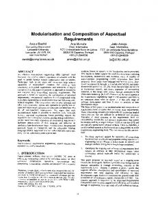
In this section, we introduce the dependence preservation and independence concatenation properties, which are necessary to join two independence relations in the right way. Dependence preservation will allow us to join an independence and a dependence relation in a correct way, whereas independence concatenation joins two independence relations taking into account that these relations after the join process may give rise to a dependence, as we will see. We begin with the discussion of dependence preservation. The reason that dependence preservation is required for joining independence statements can be explained in terms of the concepts of consistency and dominance as follows. Let the independence relations ⊥ ⊥ and ⊥ ⊥0 be defined on the same vertex set V . Then, if there 0 exist U ⊥ ⊥ W | Z and U 6⊥ ⊥ W | Z for arbitrary, mutually disjoint sets of vertices U, W, Z ⊆ V , then these independence statements and therefore independence relations ⊥ ⊥ and ⊥ ⊥ 0 are said to be inconsistent. Otherwise, the statements are consistent. The purpose is to join independence relations together; however, when two independence statements and, therefore, relations are inconsistent, a choice has to be made between the independence and dependence resulting in an inconsistence. In other words, one statement has to dominate the other one. If the relations ⊥ ⊥ and ⊥ ⊥0 are inconsistent due to the statements U ⊥ ⊥ W | Z and U 6⊥ ⊥0 W | Z, then U 6⊥ ⊥0 W | Z is said to dominate U ⊥ ⊥ W | Z. Since dominance has to be taken into account during joining independences, the following property is defined. Definition 4 (dependence preservation) Let ⊥ ⊥, ⊥ ⊥0 and ⊥ ⊥00 be independence relations all de0 fined on V . Then, if U 6⊥ ⊥ W |Z or U 6⊥ ⊥ W |Z and it holds that U 6⊥ ⊥00 W |Z for all U, W, Z ⊆ V , 00 then it is said that ⊥ ⊥ satisfies the dependence preservation property with regard to ⊥ ⊥ and ⊥ ⊥ 00 . Next, we define the independence concatenation property. This takes into account that when independence relations are combined, an independence may change into a dependence. This is demonstrated in Figure 2. In both temporal networks (a) and (b) we have that U1 ⊥ ⊥N|Θt ,Aa W3 | V3 T and U1 ⊥ ⊥N|Θt ,At W3 | V3 . However, in temporal network (a) it holds that U1 ⊥ ⊥N|Θt W3 | V3 and in temporal network (b) we have U1 6⊥ ⊥N|Θt W3 | V3 . Observe that if joining two independences results in a dependence, then this dependence is always represented by a temporal trail, which has to consist of at least one atemporal and at least one temporal subtrail. Therefore, the (in)dependence relations can be examined separately using blockage in terms of atemporal and temporal subtrails, yielding the following proposition, as basis for the definition of independence concatenation.

Proposition 1 Let U, W, Z ⊆ VT be disjoint sets of vertices and let temporal trail τ t connect vertices u and w, u ∈ U, w ∈ W , in the reduced temporal network N|Θt . If (i) one of the (a)temporal subtrails of τ t is blocked by Z or (ii) each (a)temporal subtrail of τ t is not blocked by Z but there is at least one convergent connection on two consecutive (a)temporal subtrails with vertices not included in Z, then the temporal trail τ t is blocked by Z. Otherwise, τ t is not blocked by Z. Note that Proposition 1 provides the basis for considering the case, when joining two independences results in a dependence. To ensure that these dependences are included in the new joined independence relation the independence concatenation property is defined. Definition 5 (independence concatenation) Let U, W, Z ⊆ VT be disjoint vertex sets in a temporal network N , and let G, G0 and G00 be reduced subgraphs of N with corresponding sets of trails Θ, Θ0 and Θ00 . If each trail u ∼ w, u ∈ U, w ∈ W in subgraphs G and G0 is blocked by Z and if for each q ∈ VT \ (U ∪ W ) one of the trails u ∼ q ∈ Θ and q ∼ w ∈ Θ0 is blocked by Z or these two trails do not constitute a convergent connection at q ∈ Z, then if for U ⊥ ⊥G W | Z and U ⊥ ⊥G0 W | Z, ⊥G00 satisfies the independence concatenation it holds that U ⊥ ⊥G00 W | Z, then it is said that ⊥ property with regard to ⊥ ⊥G and ⊥ ⊥ G0 .

5.2

The join operator

In this section, the join operator is defined and significant properties of this operator are given (other properties are omitted because of space limitations). We start by defining the join operator. Definition 6 (join operator) Let ⊥ ⊥ and ⊥ ⊥0 be two independence relations defined on the same vertex set V . The join operator is denoted by ◦. The join of these two relations, denoted by ⊥ ⊥ ◦⊥ ⊥0 =⊥ ⊥00 , is then again an independence relation, ⊥ ⊥00 , defined on V , that satisfies the dependence preservation and the independence concatenation properties. The dependence preservation property can be understood in terms of the union of graphs. Proposition 2 Let G = (V, A), G0 = (V, A0 ) and G00 = (V, A00 ) be three ADGs, where A ∪ A0 ⊆ A00 . ⊥G ◦ ⊥ ⊥ G0 . Then, it holds that ⊥ ⊥G00 ⊆⊥ Clearly, dependence preservation results in the property that I-mappedness is preserved. In Proposition 2 we have used the subset relation ⊆, as the resulting ADG need not precisely consist of the union of the set of arcs of graphs G and G0 . If the graph G00 equals their union and does not includes extra dependences, the join operator is said to be minimally dependence preserving. Finally, we have the following property: Proposition 3 Let ⊥ ⊥ and ⊥ ⊥0 be two independence relations defined on the same vertex set V . Then, for the independence relation ⊥ ⊥00 =⊥ ⊥◦⊥ ⊥0 it holds that ⊥ ⊥00 ⊆ (⊥ ⊥∩⊥ ⊥0 ).

6

Temporal and atemporal independence: their interaction

In Section 4, we have defined DBNs, with a graphical representation consisting of atemporal and temporal independence relations. In Section 5, the join operator has been defined such that it satisfies dependence preservation and independence concatenation. In this section, based on the two previous sections, we investigate how to employ the join operator for joining the temporal and atemporal independence relations underlying temporal networks and, therefore, DBNs, to support the modelling of non-repetitive DBNs. In Section 6.1, we show that the join operator can be used for joining the atemporal and temporal parts of the reduced temporal network. In Section 6.2, the same is shown for the atemporal and temporal relations of the entire temporal network.

6.1

Joining atemporal and reduced temporal networks

In this section, we start by the consideration of the relations ⊥ ⊥Gt and ⊥ ⊥G . Here, the following proposition establishes the connection between the d-separation relations of the individual timeslices Gt and of the set of timeslices G.

Proposition 4 Let DBN = (N, P ), with temporal network N = (VT , A), G = (VT , AaT ), A = AaT ∪ At and JPD P , then: (i) ⊥ ⊥G = ∪t∈T 6⊥ ⊥ Gt . ⊥G = ∩t∈T ⊥ ⊥Gt , and (ii) 6⊥ Proof : Case (i). The conditional independence relation ⊥ ⊥Gt consists of the complete set of conditional independences regarding its own vertex set Vt , which is, except when Gt is an empty graph, not completely included in any other ⊥ ⊥Gt0 , t 6= t0 . Therefore, the complete set of conditional independences of G is obtained by the intersection. Furthermore, the atemporal relations always describe independences between vertex sets of different timeslices. These sets of independences are the same for each relation ⊥ ⊥Gt , and these independence statements are also included in ⊥ ⊥G by means of intersection. ⊥Gt = ∪t∈T 6⊥ ⊥ Gt . 2 Case (ii). 6⊥ ⊥G = ∩t∈T ⊥ Observe that according to Proposition 4, the join operator ◦ is interpreted as the intersection of the independence relations, which does not hold in general. The connection between the join operator for reduced temporal networks is established by the following proposition. Proposition 5 Let the reduced temporal networks N|Θt ,AaT and N|Θt ,At be the atemporal and temporal parts of the reduced temporal network with independence relations ⊥ ⊥ N|Θt ,Aa and ⊥ ⊥N|Θt ,At , T respectively. Then, there exists a join operator ◦, such that the independence relation of the reduced temporal network N|Θt is equal to ⊥ ⊥N|Θt =⊥ ⊥N|Θt ,Aa ◦ ⊥ ⊥N|Θt ,At . T

Proof : Since the join operator satisfies independence concatenation and dependence preservation, joining two independence relations, the join operator has inserted all the independences, which are obtained applying the d-separation criterion. Furthermore, these two properties ensure us that there is also no incorrect relation included in ⊥ ⊥N|Θt . 2 We have joined two independence relations; however, we still have to show the correctness of the join operator in terms of the union of graphs. Soundness of the join operator means that all independence statements obtained by joining two independence relations can be read off from the union of the underlying graphs, whereas completeness means that none of the independence statements of the union of the graphs has been omitted in the resulting independence relation. Theorem 1 If it holds that ⊥ ⊥N|Θt = ⊥ ⊥N|Θt ,Aa ◦ ⊥ ⊥N|Θt ,At , then the join operator ◦ is sound and T complete. Proof : Soundness: By the temporal d-separation criterion, since the two independence relations between two vertex sets will only be joined into an independence relation, if each trail connecting these two vertex sets is blocked by the conditioning vertex set, independence in the resulting relation is implied. Completeness: We prove the completeness of the join operator by proving that if N|Θt ,AaT and N|Θt ,At are I-maps then N|Θt is also an I-map. The preservation of I-mappedness of the reduced temporal network follows from Proposition 2. Furthermore, the join operator satisfies also the minimally dependence preserving property, since N|Θt does not contain any extra arcs. 2

6.2

Joining it all together

In this subsection, the temporal and atemporal independence relations are joined together, yielding the relation ⊥ ⊥N . Recall that the atemporal relations are defined by the atemporal properties of the graph. The relation ⊥ ⊥G is obtained by the application of the concept of atemporal d-separation. Temporal relations are relations which are recovered by the temporal d-separation criteria and are denoted by ⊥ ⊥N|Θt . The following proposition shows that these relations can be linked to each other by means of the join operator. Proposition 6 Let ⊥ ⊥G and ⊥ ⊥N|Θt be atemporal and temporal independences of the temporal networks. Then, there exists a join operator ◦, such that the independence relation of the temporal network is equal to ⊥ ⊥N =⊥ ⊥G ◦ ⊥ ⊥N|Θt . Proof : Let U, W, Z ⊆ VT be disjoint vertex sets in the temporal network N . As each trail u ∼ w, u ∈ U, w ∈ W is blocked by Z then U ⊥ ⊥G W | Z ◦ U ⊥ ⊥N|Θt W | Z = U ⊥ ⊥N W | Z holds. 2 Figure 3 summarises the way to join independence relations defined in propositions 4, 5 and 6.

◦ = ∩t∈T ⊥ ⊥ Gt

(⊥ ⊥Gt )t∈T

⊥ ⊥G ◦

⊥ ⊥N

⊥ ⊥N|Θt ,Aa

T

◦

⊥ ⊥N|Θt

⊥ ⊥N|Θt ,At Figure 3: Joining temporal and atemporal independence relations. Theorem 2 If it holds that ⊥ ⊥N =⊥ ⊥G ◦ ⊥ ⊥N|Θt , then the join operator ◦ is sound and complete. Proof : Soundness follows from the temporal d-separation criterion. If each trail connecting the two joined vertex sets is blocked by the conditioning vertex set, independence in the resulting relation is implied. The proof of completeness is also similar to the proof of Theorem 1. If the relations ⊥ ⊥G and ⊥ ⊥N|Θt are I-maps then the relation ⊥ ⊥N is also an I-map according to Proposition 2. 2 Finally, the various independence relations can be compared to each other. Proposition 7 The independence sets ⊥ ⊥G , ⊥ ⊥N|Θt , ⊥ ⊥N|Θt ,Aa , ⊥ ⊥N|Θt ,At and ⊥ ⊥N also satisfy the T following properties: • ⊥ ⊥N|Θt ⊆⊥ ⊥N|Θt ,Aa , ⊥ ⊥N|Θt ⊆⊥ ⊥N|Θt ,At ; T

• ⊥ ⊥N ⊆⊥ ⊥G , ⊥ ⊥N ⊆⊥ ⊥N|Θt .

7

Conclusions

The aim of the research described in this paper was to study how the modelling non-repetitive DBNs can be simplified by distinguishing between time-independent and time-dependent independence relations. As this gave rise to various separate, but linked, independence relationships, the usual property that independence and dependence complement each other no longer holds. We introduced a join operator with special semantics to overcome this problem. Using the join operator allows one to build DBNs in a modular fashion, hence the title of the paper. As far as we know, this paper offers the first systematic method for building non-repetitive DBNs. Much work still needs to be done to bridge the gap between the theoretical work in this paper and practice.

References [1] E. Castillo, J.M. Guti´errez, and A.S Hadi. Expert Systems and Probabilistic Network Models. Springer-Verlag, New York, 1997. [2] M. Deviren and K. Daoudi. Continuous speech recognition using dynamic Bayesian networks: a fast decoding algorithm. In: Proc PGM’02, Cuenca, Spain, 2002, pp. 54–60. [3] N. Friedman, K. Murphy, and S. Russell. Learning the structure of dynamic probabilistic networks. In: Proc 14th UAI, 1998, pp. 139–147. [4] F.V. Jensen. Bayesian Networks and Decision Graphs. Springer, New York, 2001. [5] K.P. Murphy. Dynamic Bayesian Networks: Representation, Inference and Learning. PhD Thesis, UC Berkeley, 2002 [6] U. Kjaerulff. A computational scheme for reasoning in dynamic probabilistic networks. In: Proc UAI’92, 1992, pp. 121–129. [7] Y. Xiang, and V. Lesser. Justifying multiply sectioned Bayesian networks. In: Proc 6th Int Conf on Multiagent Systems, Boston, 2000, pp. 349–356. [8] A. Tucker and X. Liu. Learning Dynamic Bayesian Networks from Multivariate Time Series with Changing Dependencies. The 5th International Symposium on IDA, 2003.