Japan/US Seminar on Two-Phase Flow Dynamics December 6-11, 2004, Kyoto, Japan
On the Numerical Simulation of Acceleration-Driven Multi-fluid Mixing T.N. Dinh, R.R. Nourgaliev and T.G. Theofanous Center for Risk Studies and Safety University of California, Santa Barbara 6740 Cortona Drive, Goleta CA 93117, U.S.A. Phone: 1 (805) 893-4942; E-mail:
[email protected] ABSTRACT This paper is concerned with computational prediction of acceleration-induced multi-fluid mixing phenomena. Premises and performance of existing approaches are reviewed and analyzed with focus on a late phase behavior. We introduce a new framework whose central idea is to use an interfacial area transport equation (IATE) and a subgrid scale model (SGS) of multi-fluid turbulence to provide a natural transition from DNS-based simulation toward an effective-field model (EFM) and deeply into well-mixed states with continuous refinement of length scale. We present new results and important insights derived from our work on four platform technologies: DNS, EFM, IATE and SGS. We discuss the approach to ensure that developments in different areas effectively emerge and function seamlessly in an overall computational platform for multi-fluid mixing.
1. INTRODUCTION Accelerations on multifluid systems of unequal densities induce body force fields, and hence relative velocities, breakup, and mixing. The best known example is inertia confinement fusion, where the fluids are in gaseous form, and thus also miscible. In this case mixing gives rise to loss of temperature of the fusing component, and thus it is undesirable. Other situations can arise in fluids processing, where mixing is the pathway to creating interfacial area as needed for transfer of chemical species (extraction, reaction, etc.) or simply for dispersal and dissemination. Such situations may also involve immiscible fluids, and thus a mixing scale that is ultimately controlled by interfacial tension. One example is the dispersal and dissemination of liquids in high speed gas streams (or vice versa of high speed liquids in stationary atmospheres). In all cases we are faced with a non-stationary physical process, where the mixing zone increases with time, and where the internal (mixing) length scales evolve rapidly in both space and time. The problem has been recognized as a canonical ingredient of multifluid flow research (Theofanous and Hanratty, 2003), aiming towards a general capability (understanding and treatment) to evolving and with phase change, multifluid flow in threedimensional complex geometries. Here we are concerned with two-fluid systems, initially separated by a planar interface, subjected to an acceleration field that is directed in the same way as the fluid density gradient (or jump). This is the setting for the classical Rayleigh-Taylor instability phenomenon. It yields interpenetration: “bubbles” moving into the heavier fluid, while “spikes” shoot into the lighter fluid. The general case involves compressibility and the presence of shock waves. The special case of only impulse 1
acceleration, as the one due to a shock wave, is known as the Richtmyer-Meshkov (R-M) instability — it is inertia driven, and it leads to very similar interpenetration (mixing) behavior, but it is always active, irrespective of the direction of the acceleration vector relative to the density gradient.
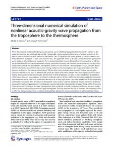
Figure 1. Numerical simulation of single-mode Rayleigh-Taylor instability (Nourgaliev et al, 2004c). Lighter fluid is accelerated into the heavier one. On the right is Planar Laser Induced Fluorescence (PLIF) image obtained by Waddell et al, 2001 in a Rayleigh-Taylor instability experiment (singlemode, miscible system). The viscid simulation was performed using a pseudo-compressible method to solve Navier-Stokes equations (Nourgaliev et al, 2004c). Numerical viscosity (diffusion) and numerical surface tension suppress short-wavelength phenomena, and fine-scale structures.
Figure 2. Numerical simulation of multi-mode Rayleigh-Taylor instability by NAR method (Nourgaliev et al, 2004c). On the right is PLIF image of multi-mode experiment by Niederhaus and Jacobs (2003) for Richtmyer-Meshkov instability in incompressible fluids. While general behavior is similar, it is evident that DNS failed to capture fine details of rolling-spike structures, due to spurious numerical diffusion. More importantly, observable differences in early stages persist on to later stages of mixing, both as self-similar behavior and as remnant from earlier spikes. Significant effect of “initial” conditions of interface on mixing and on structures of flow (vortices) was reported (see e.g., Niederhaus and Jacobs, 2003; Dimonte 2004) and analyzed by DNS for different given sets of initial interfacial disturbances (see e.g., Youngs, 2002, Dimonte et al, 2004b; Youngs 2004). The linearized R-T problem gives exponential growth of an initial perturbation, and in the absence of recognizable waves, it is assumed that the fastest-growing wave length will dominate. The non-linear regime follows quickly, as deduced from direct numerical simulations (Youngs, 1984, 1989; Glimm et al, 2001, 2003), and to some extent from non-linear analysis; it leads to interpenetrating structures (Figures 1-3) and a growth velocity (V) that is algebraic in time (see below):
V ~ c ∆ρ .a.R / ρ H
(1) 2
where a is the acceleration, R is a bubble length scale (radius), ρH and ρL are fluid densities for heavy and light phases, ∆ρ = ρH – ρL, and c is a constant.
Figure 3. PLIF images of Richtmeyr-Meshkov instability obtained by Krivets et al, 2004 (time sequence of the instability resulted from shock-acceleration by an MS = 1.27 incident shock wave). Kelvin-Helmholz instability is visible at the roll’s edges, leading to fine-scale mixing. For miscible fluids, fine-scale instability then transcends into molecular mixing (Linden et al., 1994). Noteworthy are the following: (a)
As seen in Figures 1 and 2, the internal structure of the mixing zone is only accessible by direct numerical simulations, and experimentally by a domain-cut visualization technique, such as laser-induced fluorescence (sheet illumination). The early structures show that viscous effects yield involuting, thinning layers that form into vortical structures — they are reminiscent of the vortex ball on the front edge of a penetrating viscous jet (Abramovich, 1963).
(b)
Clearly, within a penetration of a few wavelengths, the scales present in the flow vary by orders of magnitude, the small scales tending to vanishingly small, so that molecular diffusion, or in the immiscible case topological change (breakup) set in. Both mechanisms lead to variations in effective density of the media in the mixing zone, and thus one would expect an altering of the quantitative aspects of the continuing penetration of the two fronts.
(c)
As shown in Figure 2, a multimode growth leads to interference, and a higher order complexity that seems to provide a mechanism for lateral displacements of the main structures and earlier formation of occluded regions.
In the long term these structures breakup, and the mixing becomes chaotic as shown in Figure 4. This is the phase of mixing that is of the greatest interest, and it is here that understanding has resisted decades of research and very substantial commitment of resources, essentially all of it being in the context of inertia confinement fusion. What is known from experiments about this phase is that the mixing zone H grows as H = α At a t 2
(2)
3
which has been rationalized by means of Eq.(1) and a hypothesis that the effective “bubble” length scale grows in proportion to the depth of the mixing zone. In Eq.(2), At is the Atwood number defined as At = (ρH – ρL)/(ρH + ρL); and α is a factor that is apparently constant.
Figure 4. LIF images of Rayleigh-Taylor mixing obtained by Dimonte and Schneider, (2000) in Linear Electric Motor experiments. Inserts at the upper left corner are visual images of mixing zone (view from outside), which show a characteristic RTI bubble-spike structure at the boundaries of the mixing zone. The LIF images depict a highly convoluted flow pattern with a broad range of interfacial length scales. Space-wise, the interfacial length scale does not appear to be correlated with the distance from the initial interface. Theoretical/numerical work was aimed primarily at the gross features of the interpenetration (the proportionality constant α in Eq.2). Early works in DNS were that of Youngs (1984) and Tryggvason and Unverdi (1990). During the 1990s, the major efforts are still committed to DNS, although it is well recognized now that loss of fidelity due to the range of scales involved limits the applicability to penetrations of well under 10 wavelengths. At the other end, several multifluid formulations have been developed and pursued independently, with limited success, and subject to controversy (the principal ones being Youngs, 1989; Scannapieco and Cheng, 2002; Glimm et al., 2003). All that can be said with any degree of certainty is that the computations, after being sufficiently informed, have produced α values in the range 0.04 < α < 0.08 and that even these are very rough because the predicted behavior actually does not adequately conform to that of Eq.(2) (Glimm et al., 2001; Dimonte et al., 2004b). There is no understanding of what controls the internal structures, and the mixing process, nor is it known (beyond scarce and limited visualizations such as those noted above) what these structures really look like as they evolve in space and time.
4
What is apparently lacking is an appropriate framework for computation, and in this work we attempt to address this need by reaching out beyond what DNS, or Effective Field modeling, can provide individually. Specifically our principal thrust is to capture a DNS-like description within a Two-Fluid (Effective Field) model.
Each of the two fluids is resolved down to some (grid) length scale, and sub-grid behaviors are reflected by volume (or mass) fraction of the entrained (or diffused) “other” phase. Thus, each of the two fluids, seamlessly evolves from the pure phase (away from the mixing zone) to a fine (sub-grid scale) dispersion (or “solution”) of the other phase. The basic requirements, and key challenges respectively, are that the numerical scheme is able to accommodate all flow speeds, including the presence of shock waves, that volume fractions can be allowed to go to zero, thus seamlessly reducing to Navier-Stokes solutions, and that the interface treatment allows to correctly capture interfacial coupling under normal and shear stresses, as well as the production/disappearance of subgrid scale mixing, according to the local fluid dynamics. This later feature can be obtained from sample, separate DNS, which would also inform the constitutive description of interfacial area transport (reflecting the subgrid scale effective field behavior); both of these developments being also supported by experiments. We shall proceed as follows. In Section 2 we examine main models that could be considered active and of some use. We comment on issues and difficulties as we see them. In Section 3, we describe a new modeling framework. We discuss aspects of implementation and provide initial results in support of the development in Section 4. 2. MODELING AND SIMULATION APPROACHES FOR RTI MIXING: A REVIEW Due to the increasing complexity of flow patterns during a later phase of the RTI mixing, analysis strategies other than DNS must be developed. This need was recognized in 1980s and pioneered by Youngs (1989). Clearly, presence of multiple interfacial length scales in the mix zone renders coarsegraining inevitable. Progress of understanding and developments in the field of RTI and RMI mixing can be found in Brouillette (2002), Zhou et al (2002, 2003) , Cabot et al (2004), Cheng et al (2003, 2004). In the present review, we discuss relative merits of different approach, ranging from Large Eddy Simulation (LES) model, to turbulent mix model (TMM) and to two-fluid, effective-field model (EFM); the former two approaches are focused on the turbulence behavior, while the latter is anchored on the notion of two interpenetrating continua. Single-Fluid Turbulent Mix Model This approach, with a number of variations in detail formulation, is a natural extension from Direct Numerical Simulation (DNS) for single-fluid flow. It is based on solving the Navier-Stokes equations and then using a scalar transport equation to follow phase distribution. For instance, Young (1984; 1989) solve a transport equation for volume fraction, α (for one fluid, and (1-α) for the other fluid): ∂t α + div (α U) = 0
(3)
while Cabot et al. (2004) solves a convective-diffusive transport equation for local mass fraction c for one fluid with density ρ1, where (1-c) for the other fluid with density ρ2: ∂t (ρc) + div (ρcU) = div(ρD∇c)
(4)
Here D is the coefficient of diffusivity. The mixture density ρ is defined as
5
ρ = 1/ (c/ρ1 + (1-c)/ ρ2)
(5)
Notably, equations (3) and (4) constitute heuristic models of mixture transport. The modeling content (homogenization) is further included through the use of “innocent”, yet heuristic relations which relate the mixture’s properties to phasic properties; e.g. see Eq.(5). Further, Cabot et al, 2004 implemented a subgrid scale model, taking computational advantages of LES over DNS to bring simulations to a later phase of RTI mixing. Broadly speaking, the LES concept has evolved from an early version of “static” subgrid scale (SGS) model by Smagorinski (1963), Moin and Kim (1982) to more sophisticated dynamic models, e.g. Germano (1992), Ciofalo (1994), Jaberi and Colucci (2003). Application of LES to multiphase flow is a new field, with focus placed on particulate and bubbly flows; see e.g. Dean et al. (2001), Lakehal et al (2002), Apte et al. (2003).
Major uncertainties remain with formulation of subgrid scale models in anisotropic, variable-density flow. Even attempts to use “DNS” to benchmark LES should be treated with a great care, because “DNS” in multi-fluid flow are not first-principle calculations because of heuristic elements represented by Eqs. (3-5). In general, formidable challenges exist in turbulence modeling in RTI mixing, and especially in RMI mixing; a recent review of progress made in this area, including turbulent mix model, is provided by Zhou et al, 2003. Remarkably, the mixing zone flow pattern evolves from a quiet, low-Reynoldsnumber state into an intense mixing, requiring the turbulence model to function over a broad range of conditions. The unsteady and anisotropic nature of RTI/RMI mixing makes single-point-closure (spectral equilibrium) models inapplicable, as shown by DNS results of Cook and Zhou, 2002. In response, multiple-time-scale turbulence models were considered (Souffland et al., 2002; Zhou et al, 2002; Zhou et al, 2003); but they even require a larger number of closure constants. In addition, lack of data and understanding on the effect of compressibility on turbulence further hampers the treatment of RMI mixing. Two-Fluid Turbulent Mix Model Works on two-fluid modeling for RTI/RMI mixing during 1980-1990 capitalized on parallel efforts to develop the theory and computation of multi-fluid flow; see e.g. Ishii, 1975; Drew, 1983; Drew and Passman, 1998. Early references for two-fluid turbulence modeling of Rayleigh-Taylor mixing dated back to Youngs (1989), who referred also contemporary works in U.K. by Spalding (1987) and Andrews (1986). They used conservation equations of an interpenetrating continua model in conjunction with a point-closure turbulence model, e.g. k-L, or k-ε model. To a significant extent, Youngs’ model resembles the disperse flow model developed for bubbly and particulate flow (e.g., see Lahey and Drew, 2001 and earlier references cited therein). Notably, Youngs’ two-fluid modeling approach has hardly taken off the ground in RTI/RMI mixing applications. The reason is dual. On the formal side, large uncertainties in the model’s closure under the RTI/RMI mixing conditions, both for turbulence and for inter-phase interactions, diminished the model’s predictive capability. On the substantial side, the disperse-flow-like approach does not offer a framework to effectively model a key physics of RTI mixing, namely the continuous refinement of length scale. Recent attempts to remedy the situation include a two-structure, two-fluid, twoturbulence model of Llor and Bailly (2003), Llor et al (2004) who relate geometrical length scales in the turbulent mixing zone to turbulent length scales. The success in Llor’s (2003, 2004) and similar efforts to invoke physical arguments and integral measure to improve two-fluid model closures is yet to be seen. 6
Glimm’s Chunk Mix Equations and Buoyancy Drag Model The practical need to perform analysis of mixing dynamics in RTI and RMI as part of another, multifaceted process (e.g., inertial confinement fusion implosion) motivated Glimm and co-workers to develop a special class of two-fluid model. The approach, some time called chunk mix equations, was pioneered and advanced in Glimm et al. (1998, 1999, 2003), Saltz et al. (2000, Cheng et al. (2003). In their recent paper Glimm et al. (2003) continued to build upon their previous developments of the two-pressure chunk mix model (Chen et al., 1996; Cheng et al., 1999, and other references cited in Glimm et al., 2003). Notably, they separated, and in effect totally decoupled, the mix and unmixed regions; the two-phase model describes the mix region with moving boundaries; the latter are prescribed as a closure law or the so-called buoyancy drag model. The two-fluid model equations used in Glimm et al (2003) were said to be obtained by an averaging procedure. Remarkably, a volume fraction transport equation is used ∂t α + v* ∇α = 0
(6)
which presents an averaged version of microscopic interface equation (Drew and Passman, 1998). At its basics, Glimm et al (2003) model is similar to Ransom and Hick (1979) model for stratified flow and to a better known Baer and Nunziato, (1986) model for multiphase combustion. Properties of models of this class were discussed in Dinh et al., 2003. Other works related to Baer-Nunziato model worthy mentioning here include a discrete equation model (DEM) for compressible multiphase mixture derived by Abgrall and Saurel (2003) and its extension with “internal degrees of freedom” by Saurel et al (2003). In all cases, the models include the volume fraction transport equation (VFTE, or also called compaction dynamics equation in Baer and Nunziato, (1986) model). The VFTE requires modeling of mixture/interface velocity v*, (Glimm et al., 2003) v* = β1 v2 + β2 v1
(7)
The volume fraction transport equation (VFTE) is an averaging version of phase index equation similar to a level set equation for phase interface. A global view of the VFTE, combined with the two-fluid model, indicates that this VFTE equation is redundant for mass conservation equation. Furthermore, the VFTE does not provide the interfacial area, which depends on two-phase pattern (in-cell structure). The latter information is lost in the homogenization procedure. A close-up view of VFTE indicates that high spatial resolution (small control volume or grid size) enables a strong correlation between volume fraction and interfacial area. However, such close-up view is in conflict with the notion of volume fraction as a probabilistic measure of phase index.
Interestingly, by the virtue of this additional modeling equation, all eigenvalues of the two-phase flow model used in Glimm et al (2003) are real. One advantage of this model using VFTE is that although the model is non conservative and not strictly hyperbolic (not all eigenvalues are distinct), experience shows that numerical methods developed for hyperbolic conservation laws can easily be adopted for solving the model equations. Physically, Glimm et al (2003) two-phase model differs significantly from alternate two-fluid models, in the sense that the former does not recognize interfacial length scales. This removes the need to consider turbulent structures and their role in inter-phase momentum exchanges. However, the model’s underlying fundamental assumption about the “mixing zone homogeneity” is in conflict with experimental observations (see Figure 4 for example) and with the flow regime described by Glimm et al. (2003) as “characterized by large scale coherent mixing structures … on the order of the thick ness of the mixing zone”.
7
In summary, Glimm and co-workers have brought the effective-field modeling in RTI mixing to a new level of mathematical sophistication. Clearly, the hope is that mathematical consistence between a two-phase model with edge-moving models, closure expressions and interface-velocity model may be sufficient to capture dynamics of RTI mixing, thus circumventing the need for detail knowledge of turbulent structures, length scales etc. This way the approach does not give new insights into the physics of mixing, which is instrumental for a two-phase model to be used as a predictive tool. Scannapieco and Cheng (2002) Multifluid Interpenetration Mix (MIM) Model Scannapieco and Cheng (2002) derived multifluid momentum equations from the collisional Bolztmann equation, resulting in only one phenomenological quantity, i.e. the collisional frequency, which describes unresolved physics (mixing/interaction). According to Scannapieco and Cheng (2002), their model is a generalized form of hydrid turbulent mix model developed during 1991-1992 by C.W. Cranfill at Los Alamos National Laboratory. We note that the resulting model includes mass, momentum and energy conservation equations for mixture’s variables, such as the mass-mean bulk flow velocity v*. The model also includes a transport equation for phasic density, or equivalently concentration (of species s). This equation includes the effect of fluctuating velocity 〈US〉, and this is a unique feature of the Scannapieco and Cheng (2002) model. The model is closed by a two-equation turbulence model, namely the transport equations for the fluctuating velocity and kinetic energy density eS measured in a frame moving with the bulk fluid v*. Thus, the model is globally equilibrium while allowing for local (mechanical) non-equilibrium in the sense that two fluids have the same “bulk” velocity while featuring different fluctuating velocity. Given a robust numerical scheme to solve its sets of balance equations, one can expect the MIM model to provide a natural transition from unmixed through initial mixing phase and deep into mixing. The edge (mixing zone front) may be implicitly captured by the phasic density transport equation. In our view, due to the nature of assumptions on which the model was derived, it is suspected the MIM model is less applicable to more traditional conditions of RTI and RMI mixing, but suits better intense mixing conditions. On the one hand, no direct experimental validation of the Scannapieco and Cheng (2002) model against “classical” RTI and RMI experiments is available in the literature. On the other hand, Wilson et al (2004) reported using this multifluid interpenetration mix model to describe mixing in directly driven inertial confinement fusion capsule implosions and found a good agreement with experimental data. More interestingly, it was found that the model’s only parameter is robust under different test conditions (fuel pressures). It was also suggested that this single mix parameter can be used to model symmetric and asymmetric implosions. 3. A COMPUTATIONAL FRAMEWORK FOR MULTI-FLUID MIXING 3.1. Basic requirements Complexity in RTI and RMI mixing phenomena is manifested through multiple and variable length scales which evolve in the mixing zone. In the previous section, we discussed different coarse-grained modeling approaches built on different assumptions about the nature of these length scales, their relative dominance, their spatial distribution (interior region vs. buoyancy drag edge regions). Methodologically, one can see these efforts as either bottom-up and top-down. The bottom-up approach focuses on the initial stage, viewing interfacial instability as the mixing’s driving force. Consequently, DNS prevails, using a subgrid scale model (LES) to compensate for well-mixed states. The top-down approach emphasizes the late stage of phase interpenetration, putting the multifluid model to the center. In both approaches, there exists a host of subgrid-scale physical phenomena that requires modeling, from molecular mixing to micro-mixing during interfacial breakup. The DNSbased approach needs to go beyond a simplistic transport equation for mass concentration or volume 8
fraction; even in the early stage of instability, the “mix” should be allowed to emerge, evolve and interact with the “main” fluids; see Figure 5. Notably, the buffering “mix” influences momentum (and energy) interaction between two “main” fluids. Failure to account for the buffer effect leads to accumulation of errors and eventually wrong solutions.
Figure 5. Two-fluid mixture is generated at the fluid-fluid interfacial region due to instability and breakup, and under-resolution in experimental imaging and in numerical simulation. Microscopically, the “mix” should necessarily be two-fluid. It is because even when the “mix” mass-mean parameters are in equilibrium, thermal and mechanical fluctuations of separate fluids may well remain nonequilibrium. Furthermore, in practice, fluids participating in mixing not only feature distinctive “functional” properties (e.g., reaction rate, viscosity), but their thermodynamic properties (including equation of state) may differ significantly. Macroscopically, the “mix” is also far from homogeneous even in a seemingly one-dimensional RTI-induced mixing. Our examination of experimental images (Figure 4) suggests that large scale structures emerge and persist throughout the mixing process. We also note the structure’s length scales in the later phase being characteristically larger than wavelengths of the initial interfacial instability. Therefore, the remnant effect from the initial instability alone can not explain the origin of the large-scale structures. Such flow patterns may emerge from dispersed systems – a behavior known and discussed previously (Theofanous and Dinh, 2002; Dinh et al, 2003).
Figure 6. Filtering in multifluid mixing. 9
In light of the above remarks, we envision that RTI/RMI mixing phenomena are best numerically simulated in a multi-fluid framework, which provides a natural, smooth transition from DNS-like description for supra-grid fluid motions to the two-fluid model for sub-grid-scale (SGS) fluid transport; see Figure 6. The grid size ∆ thus serves the filtering width. The concept’s basic idea is very similar to that of the LES, with a key difference being the SGS multi-fluid actions are described by transport equations instead of being treated in a local equilibrium formulation characteristic of the LES. Furthermore, since under RTI/RMI mixing flow the interfacial length scale is continuously refined and transported, we propose to use an Interfacial Area Transport Equation (IATE) to provide a physics-based closure for the model; see Figure 7. It is important to contrast VFTE with IATE. The Volume Fraction Transport equation (VFTE) deals with volume fraction, which is directly related to conservation variables in LHS, whereas the Interfacial Area Transport Equation (IATE) deals with a parameter in constitutive relations (RHS). As such, the IATE does not explicitly enter the differential structure of the two-fluid model.
It is essential for the successful implementation of the proposed framework that it is supported by multi-dimensional numerical schemes which “walk” seamlessly from DNS-type single-fluid regions to the mix, and again, across the mix’s boundaries toward unperturbed single-fluid regions. This means the mixing zone’s boundaries should be captured automatically, instead of being explicitly tracked by a foreign correlation-based model. Derived and validated against specific experiments, such a semi-empirical model has limited predictive capability in situations of practical interest. More importantly, the correlation-based approach is one-dimensional. This is contrasted with threedimensional phase distributions observed at the mix’s boundaries; see Figure 4, and also see Srebro (2003). We believe that the ability to capture the emergence and evolution of such instability-like structures is essential in predicting the late-phase mixing dynamics.
Figure 7. The proposed framework for effective-field modeling of turbulent multifluid mixing.
10
Mathematical Formulation: a Two-Fluid Model with IATE and Transported LES Our current modeling effort is anchored on the “classical” set of conservation equation of the twofluid model as derived in Ishii (1975), Drew (1983), Drew and Passman (1998). Reynolds averaged conservation equations for (k)-field with volume fraction α(k) (Σα(k) = 1):
∂ t ρ( k )α ( k ) + ∂ j (u( k ) j ρ( k )α ( k ) ) = S((kρ))
∂t (u(k )iα(k ) ) + ∂ j (u(k )iu(k ) j ρ(k )α(k ) + P(k )α(k )δij ) = P( I )∂iα(k ) + ρ(k )α(k ) gi + S((ku))i ∂t (E(k )iα(k ) ) + ∂ j ((E(k )iα(k ) + P(k )α(k ) )u(k ) j ) = −P(k ) ∂tα(k ) + S((kE))
(8-1) (8-2) (8-3)
where ρ(k), u(k)j , P(k) and E(k) are density, velocity, pressure and energy of the k-fluid. Separate equations of state are used for each fluid, which relate ρ(k), P(k) and E(k). The compatibility condition states
∑α
k =1, 2
(k )
=1
(8-4)
ρ
Source terms S( ), S(u) and S(E) represent both inter-phase exchanges and diffusion contributions. Of important for the RTI mixing modeling is
S (u)(k) = ∇.[α(k) (µ(k) + µ T(k)) ∇u(k)] + I(k)
(8-5)
Where the first component in the RHS represents diffusive transport, both laminar and turbulent, and the second component (I(k)) represents an inter-fluid friction force as it arises from relative motion of the two fluids at the sub-grid-scale level. Generally, I(k) depends on the relative phasic velocity (∆u = u(1) – u(2)), on characteristic length scales of interfacial contact, and the phasic volume fraction. The latter two variables can be effectively represented by a so-called interfacial area density A. The later is varied for different flow regimes. As a special case, when volume fraction of one fluid vanishes (and that of the other fluid reaches unity, i.e α(k) = 1), I(k) → 0 and Eq.(8) can be transformed into a Reynolds-averaged Navier-Stokes equation for k–th fluid; see Figure 7. Denoting A(k) as interfacial area density for k–th fluid, IATE has the following form (Ishii et al, 2002) (9) ∂t A(k) + div (A(k)u(k)) = S (A)(k) where source term S represents rates of interfacial change due to coalescence or breakup. In the RTI/RMI case, this source term is positive due to continuous refinement of length scales (breakup). Relating this source term S (A)(k) to local phasic distribution and flow conditions is a key research task, which determines the success of the whole modeling framework. A robust treatment of S (A)(k) must build upon a host of fundamentally-oriented, advanced-diagnostic experiments, computations (DNS) and theoretical analyses. (A) (k)
11
Turbulent viscosity µT in Eq.(8-5) can be determined from a subgrid scale turbulence model which describes turbulent contributions at the far-end spectrum (in the LES spirit). A straightforward pathway is to make use of existing single-fluid LES models, such as that of Smagorinski (1964) or Germano (1992). Since the k–th fluid occupies only a fraction α(k) of control volume, the LES model should accordingly be factored by α(k). In effect, this solution renders “stratified” two fluids within the control volume with respect to turbulence stress, whereas the interfacial structure is accounted for in the interfacial stress to I(k). Due to the nature of directed transport in RTI and RMI mixing, we suggest and recommend another approach, named here as a “transported LES” model, to determine µT. The idea is to make use of well-developed K-ε formulations for modeling of turbulent disperse particulate and bubbly flows; see e.g. Elghobashi, and Abou-Arab (1983); Zaichik et al. (1997); Lahey and Drew (2001). Specifically, additional scalar transport equations are used to compute kinetic turbulence energy K and its dissipation rate ε for each fluid. Turbulent viscosity can then be determined by
µT(k) = Cµ ρ(k) [K(k)]2 /ε(k)
(10)
Although the proposed “transported LES” model has a similar structure of Youngs (1989) model (i.e using a two-equation, k-ε or k-L, model for turbulence transport), a major conceptual difference exists between them. In the present work, a high spatial and temporal resolution must be used in computations to ensure that all of the under-resolved subgrid-scale turbulence belongs to the far-end high-frequency region of turbulence spectrum. In the contrary, the Youngs’ model was tuned to cover spectrally averaged, energy-containing vortices. Furthermore, we use IATE to follow the interfacial length scale – an aspect not covered in Youngs’ (1989) model. 4. IMPLEMENTATION OF THE NEW FRAMEWORK. INITIAL RESULTS. Having addressed conceptual bottlenecks in existing approaches for multi-fluid mixing (particularly for RTI and RMI mixing), the proposed framework also presents significant challenges for its practical implementation. The new framework requires new kinds of numerical treatments as well as physical models for closure, as compared to previous works in this area. Figure 8 depicts four main topical areas that need attention, namely 1. 2. 3. 4.
DNS-based computational technology, Two-fluid modeling and numerical solution, Realization of the interfacial area transport equation under continuous refinement of length scales (mixing), and Subgrid-scale turbulence model in two-fluid setting.
Individually, these areas have been studied, developed, and applied to multiphase flow simulations. Areas (1) and (2) present the mainstream of activities in RTI/RMI mixing studies. Areas (3) and (4) have been developed and applied more in the context of disperse flow than for mixing flow. Most importantly, for the present purpose, the four Areas need to be addressed in a consistent manner, so for the resulting developments in individual Areas to function seamlessly in the overall framework for multi-fluid mixing.
12
Figure 8. Topical areas, tasks and challenges in implementation of the proposed framework for modeling of multi-fluid mixing.
Figure 9. Approach and building blocks of the implementation.
13
Figure 8 also summarizes major tasks and challenges in each area. Further, Figure 9 shows our approach and building blocks we need to have to meet the challenges. In the remaining of this paper, we will discuss the tasks and the approach. Arrows in Figure 9 indicate areas where a more detailed review of the state of the art and our new results are given. Area 1: DNS and fluid-fluid interface treatment Within the proposed modeling framework, DNS capability is the starting point. The DNS-based method is needed for the accurate simulation of the initial phase of instability and mixing. In case of RMI, the instability results from complex interactions of pressure shock waves with interface between two fluids (with different acoustic impedance). It is critical to both effectively capture the evolving interface and robustly treat information flow across such interfaces. There exists panoply of methods developed for this purpose. Front-capturing (e.g., level-set, ghost-fluid) methods offer flexibility in handling complex geometries, whereas front-tracking techniques capitalize on the use of Riemann solution at the multi-material interface to achieve high accuracy. Interestingly, Fedkiw et al (1999) pioneered the idea to incorporate a Riemann solution into the ghost-fluid method for accurate treatment of discontinuity (in detonation). Later, effective treatment of high acoustic impedance mismatch interface (gas-solid, gas-liquid) was also achieved in the revised Ghost-Fluid Methodology by Fedkiw (2002).
Figure 10-a. Mixing of helium gas cylinder (“bubble”) with air upon a shock (shock Mach = 1.22, right-to-left). Experimental images are by Haas and Sturtevant, 1987. On the right of the experimental images are computational images obtained by the present authors using DNS (Nourgaliev et al., 2004). Although instabilities appear to occur on the “bubble” surface, fluid-fluid contact is treated in this DNS as an ideal interface. Excellent agreement between experimental observation and computational result is achieved for overall bubble behavior and shock structure. In our works, we develop a hydrid method, named Characteristics-Based Matching (CBM); block 1.1.b; see also Nourgaliev et al (2004). The CBM is designed to bring out best features of the frontcapturing and front-tracking methodologies, in a unified fashion over generic multi-material interfaces; see Nourgaliev et al. (2004a). Figures 10-11 illustrate the performance of the CBM methods against unique experimental images obtained by Haas and Sturtevant (1987). Notably, Haas and Sturtevant (1987) experiments have been considered as benchmark tests for multi-fluid DNS methods, aiming to predict complex flow phenomena in Richtmyer-Meshkov instability.
14
Numerical results similar to that shown in Figures 10-11 were previously obtained by Quirk and Karni (1996) using Adaptive Mesh Refinement (AMR) algorithm. They used a weighting scheme (e.g., Eq.5) to treat the interfacial region. In a way, the treatment provides an account for parabolic behavior at the boundary layer (refined region near interface). The good agreement between DNScomputed results (both in Quirk and Karni, 1996 and Nourgaliev et al., 2004a-b) and experimental observations indicate that until the interface becomes convoluted and broken up, the DNS-based method is an appropriate tool for early stages of mixing. For a later phase, experimental images indicate a fine-scale mixing, for which the DNS–based “sharp-interface” representation is inadequate.
Figure 11. Mixing of R22 gas “bubble” with air upon a shock (shock Mach = 1.22). Experimental images are by Haas and Sturtevant, 1987. On the right of the experimental images are computational images obtained by the authors by DNS (Nourgaliev et al., 2004a). A good agreement between experimental observations and DNS results is achieved for the initial phase. In a recent work (block 1.1.a), we combine the level-set algorithm with another advanced solver – the AUSM+up method developed by Liou and co-workers; see Liou (1996); Liou and Edwards (1999, 2003) Chang and Liou (2003, 2004). Most notably, Chang and Liou (2004) showed that a novel AUSM treatment enables using the two-fluid formulation to perform DNS-like multi-fluid computations when volume fraction of one fluid (phase) in some sub-domain vanishes (such as in the gas or water column of Figures 10-11). Another key ingredient in DNS-based computation of multi-fluid flow is the capability to accurately preserve structures and track masses as the structures get thinner. Numerical viscosity and numerical “surface tension” are known to reduce accuracy. Their effect can become dramatic in certain flow conditions. An example is a shear layers with formation of rolling structures; Figure 12 (left). Indeed, one can observe a striking similarity between the roll in shear layer and the one observed in 15
Richtmyer-Meshkov experiment (Niederhaus and Jacobs, 2003.). Not surprisingly, we found that formation of spurious structures is sensitive to both the grid resolution and to the numerical methods used. Methods based on Cartersian grids (AC and PRJ in Fig.12) have dominant directions along the grids, whereas the dominant flow direction is somewhat diagonal. Consequently, spurious vortex is created. No such spurious vortex is seen in simulation by MRT scheme based on lattice Bolztmann equation method, which has eight velocities (in 2D) including the diagonal ones.
Figure 12. Numerical simulation of a double shear layer using different numerical schemes: MRT: multiple relation time scheme of a lattice Bolztmann method; AC: high-order artificial compressibility scheme (Nourgaliev et al., 2004c), and PRJ4: fourth-order accurate projection method. Spurious velocities and vortex detected in AC and PRJ solutions with low numerical resolutions are removed at a higher resolution. The lattice-Bolztmann equation MRT method shows a resistance to formation of spurious vortex. The right insert is an LIF image of incompressible Richtmyer-Meshkov instability experiment by Niederhaus and Jacobs, 2003. A striking similarity of rolling flow patterns is depicted. It is noted that in the previous example (Figure 12) all methods can be made to eventually provide solutions with a reasonable accuracy as we refine the computational grid. Such an approach is inefficient in capturing distinct structures (Fig.12) and unrealistic for simulation of complex flows, such as in RTI/RMI mixing. This necessitates the application of adaptive mesh refinement (AMR) methodologies, and we have made significant progress in this direction (Nourgaliev at l., 2004d; 2005a-b). We use a platform technology SAMRAI developed in Lawrence Livermore National Laboratory; see Wissink and Hornung (2000), Wissink et al (2001). An example of efficacy and accuracy that can be achieved with AMR is shown in Figure 13. Without sufficient grid resolution and AMR, under-resolved fluid is numerically dissolved, leading to a so-called mass loss in the level set treatment. In mixing flow, the “mass loss” matter is further complicated by the dual cause of the mass loss: physical origin related to instability-induced breakup and fluid entrainment, and numerical origin due to under-resolution of interfacial curvature and length scale. The physical mechanism gives rise to the subgrid-scale “mix”. A bridge between the DNS-based computations and the two-fluid description is provided through in the interfacial area transport equation (block 1.2.a) . In particular, generation of the “mix” can be described by a physics-based source term (entrainment) in interfacial area transport equation (blocks 3.2.a). 16
Figure 13. Deformation of a circular (2D) body in a rotational flow field as described by a level set algorithm. First and third columns are results for uniform grid. Second and fourth columns are results for adaptive mesh refinement (AMR), using three levels of grids (SAMRAI platform; Wissink, and Hornung, 2000; Wissink et al., 2001). Significant reduction of mass loss and preservation of structures are obtained when AMR is used (Nourgaliev et al., 2004d, 2005b). Area 2: Two-fluid modeling and numerical treatment The two-fluid model is the main computational vehicle in the proposed framework for multi-fluid mixing. The review in section 2 readily indicates a large body of knowledge and experience on the theory, computations and applications of the two-fluid model. Despite their common name (twofluid), specific two-fluid models differ in their physical basis, mathematical property and issues in numerical treatment. For example, Glimm et al (2003) include Eq.(6) (VFTE) in the differential operator of the two-fluid model, rendering all real eigenvalues and making the two-fluid model hyperbolic. Although attractive mathematically, such a modeling approach is intrusive and does not reflect an essential attribute of the mixing process, namely the continuous refinement of length scales. In the proposed framework, we use Eq.(9) – the IATE – to close the system. Since Eq.(9) does not enter the differential operator, it does not serve to regularize the two-fluid model equations. Derived from a homogenization procedure, the two-fluid transport equations are known to be illposed and mathematically complex, in the sense that the equation system is non-hyperbolic, nonlinear and non-conservative; a comprehensive review and analysis of the ill-posed two-fluid model can be found in Dinh et al (2003). Furthermore, the two-fluid model employs constitutive laws of inter-field interactions for closure. Large uncertainties exist in determining inter-field exchanges in compressible systems because non-local (long-range) nature of the interactions. As a result, fidelity of multi-field numerical solutions is confounded by the interplay between phenomenological uncertainty in mostly empirical constitutive laws and numerical errors due to numerical diffusion and unphysical oscillations; see Figure 14.
17
This above-discussed issues all go to the heart of the “consistent treatment” of the four Areas in the proposed framework (Figure 8), because both interfacial area transport equation and its source terms (Area 3) and sub-grid scale turbulence transport (Area 4) are brought into this framework to provide physics-based closures and regularization for the two-fluid model (Area 2).
Figure 14. Water faucet problem. Numerical solution of conservative, non-hyperbolic two-equation systems of the two-fluid model. Numerical (oscillatory) and analytical (vertical front propagation) solutions are given for time moments t = 0.2s, 0.4s, 0.6s, 0.8s, and 1.0 s. Dinh et al (2003). One must-have attribute in the two-fluid treatment of multi-fluid mixing is the model’s ability to capture structures (clusters), shocks and discontinuities as such inevitably emerge and control the mixing dynamics. Only recently, progress in mathematics analysis of hyperbolic conservation laws, including multidimensional conservation laws and not-strictly-hyperbolic equations such as that of the two-fluid model (e.g., Keyfitz, 2001, Keyfitz et al., 2003; for review see Dinh et al., 2003) suggests that the two-fluid model differential operator may readily embed the complexity; yet the emergence of complexity requires special care in the model’s numerical treatment, which in turn demands the model be hyperbolic and well-posed. Within the proposed modeling framework, it is essential that the two-fluid solution be achieved on a high-definition grid, rendering a higher degree of anisotropy for sub-grid turbulence and a higher degree of homogeneity for sub-grid phase distribution. However, as the grid refines, numerical solutions of the ill-posed two-fluid model become unstable and disconverge; e.g., see Nourgaliev et al (2003); Dinh et al (2003). We have also showed that stable, convergent solutions can be obtained when the equation system is regularized to hyperbolic (Figure 14). That convergent solutions can be obtained for hyperbolic two-fluid systems is consistent with the Glimm et al.’s work on another twofluid model (with VFTE). However, we use a local, algebraic correction to reach hyperbolicity, instead of using the differential equation (VFTE) for this purpose, as in Glimm et al (2003). Interestingly, our analysis suggests that the two-fluid model’s ill-posedness is not a mathematical artifact; we relate the ill-posedness to the loss of “structural” information upon the homogenization Dinh et al (2003). The degree of ill-posedness is therefore defined by the role and effect of the lost, filtered-out, sub-grid-scale information on the collective, global flow behavior described by the averaged field equations. The relative importance of the filtered-out information increases when the filtered-out, anisotropic behavior becomes nonlinearly coupled with the grid-scale phenomena. Such
18
situations must be identified, and their treatment will likely invoke the notion of flow regimes, to take into account structural information of flow pattern (block 2.1).
Figure 15. Results for the water faucet problem. Numerical solution of non-conservative, hyperbolic two-equation systems of the two-fluid model. 20000 cell grid. Numerical and analytical solutions are given for time moments t = 0.2s, 0.4s, 0.6s, and 0.8s. The equation system is made hyperbolic by a socalled “interfacial pressure term”. Dinh et al (2003) showed that the origin of such term is not physical (no relation to interfacial pressure) but mathematical. Its formula represents what is needed to bring the equation system to the hyperbolicity, thus reflecting the degree of non-hyperbolicity of the two-fluid model. With respect to regularization of the two-fluid model, a recent development of the AUSM+up method for two-fluid simulation deserves attention. The AUSM+up method belongs to the AUSM (Advection Upwind Splitting Method) family pioneered by Liou (1996); see also Liou and Edwards (1999, 2003). One of the attractiveness of the AUSM schemes is that they do not need characteristic decomposition (i.e. determine the system’s eigenvalues), thus significantly simplifying the algorithm, as compared to, for example, a characteristics-based method developed in Nourgaliev et al. (2003). Notably, Chang and Liou (2003) showed that they can achieve stable and convergent solutions of the two-fluid model equation systems in a number of benchmark tests, including the water faucet problem. Specifically, Chang and Liou (2003) employed a hyperbolized two-fluid system with the “interfacial pressure” term. Another key feature of Chang and Liou (2003) work is the derivation of a high-order flux that takes into account inter-cell, inter-fluid interactions in an one-dimensional stratified flow configuration. The “stratified” scheme was extended in Chang and Liou (2004) for two-dimensional simulations, simply by using a dimension-by-dimension treatment. It is noted that, on the one hand, the notion of stratified flow in flux treatment provides a way to account for sub-grid scale multi-fluid structure (lost in homogenization and causing ill-posedness). On the other hand, injection of a specific flow pattern into the scheme prior to solution violates the objectivity principle in the effective-field (homogenized) model. Currently, our work (block 2.2; Figure 9) includes analysis of mechanisms by which the new AUSM flux treatment influences the numerical solution of the two-fluid model equations. The work also includes extending the AUSM flux treatment scheme to other flow patterns, and developing a methodology to select appropriate schemes.
19
Area 3: Interfacial area transport equation and source terms This area is central in the new framework. The first, important question is related to the formulation of the interfacial area transport equation itself, namely the use of material velocity u(k) for in Eq.(9); block 3.1. It is not obvious that in RTI/RMI situations (with mean flows being counter-current) the material velocity is adequate approximation for the “interface transport” velocity. The formulation should be assessed by DNS, first for counter-current disperse flow, and then for mixing flow (i.e. with interfacial breakup).
Figure 12. Aerobreakup of liquid drop suddenly exposed to a supersonic gas flow (Mach 3). Evolution of interfacial area with multiple length scales is evident. A close view shows instabilities on drop surface and formation of mist of broken mass (Theofanous et al, 2004). The other sub-area (block 3.2) is related to source terms in Eq.(9) – representing the creation of interfacial area in multi-fluid mixing. The objectives in this sub-area are to develop constitutive laws for rates of interfacial area generation as function of local flow conditions and phase distributions. For the initial transition from single-fluid DNS behavior to mixture, the interfacial area generation rate can be evaluated using existing models and available data for liquid entrainment and deposition (block 3.2.a). This approach is akin to the treatment of Large Scale Discontinuity proposed and discussed previously in Dinh et al (2002).
20
For interior mixing (block 3.2.b), the internal length scales are obscure for observation. To obtain insights and data on interfacial area generation rates in such interior mixing, one must develop advanced diagnostics, perhaps a combination of penetrating/attenuating radiographic methods and computer tomographic techniques. The importance of diagnostics of multiphase flow regime was previously discussed in Theofanous and Dinh (2002) and Hanratty and Theofanous (2003). Clearly, development of a credible database and understanding for interfacial area generation and transport in multi-fluid mixing requires a comprehensive experimental program, ranging from fundamental experiments of liquid drop breakup to RTI/RMI mixing experiments (blocks 3.2.c-d). In particular, we have been focusing on breakup behavior of a liquid droplet exposed to supersonic flow (Theofanous et al., 2004). High-speed, high-resolution images obtained in our ALPHA experiments in a supersonic pulse wind tunnel give powerful new insights. The data reveal that drop deformation and breakup are governed by Rayleigh-Taylor instability at low Weber numbers, while shearing and stripping enter more intensely with the increase of Weber number. The visualization and image processing techniques enable determining the particle size distribution, which is essential for the characterization of the rate of mixing and interfacial area generation. Area 4: Two-fluid, sub-grid-scale modeling of turbulence transport Work in this topical area benefits from advances made in understanding and modeling of two-phase flow turbulence in disperse systems. Note that past studies were directed to uniform-size particulate flows or fairly dilute bubbly flow, where the effect of collision, coalescence or breakup can be neglected. Studies on bubbly flow that account for coalescence and breakup are limited to the treatment of interfacial area density (Ishii et al., 2002) . No studies were found to have addressed the two-fluid turbulence behavior in systems with rapid refinement of length scales (intense mixing conditions). Therefore, the first challenge for turbulence modeling in multi-fluid mixing is to derive two-fluid sub-grid scale turbulence transport model, which is consistent with the IATE treatment (block 4.1; Figure 9). In section 3, two approaches – the traditional local-equilibrium LES model modified to volume fraction and the transported LES – were considered. Implementation of the localequilibrium LES is straightforward. For transported LES, the use of AUSM-based numerical scheme allows for an easy implementation of additional scalar transport equations. The task (block 4.1.b) is to examine the relative performance (trends) of the two formulations. The other challenge is to quantify constants needed in the turbulence model. Fundamentally-oriented, physical and numerical (DNS) experiments provide the central avenue in this area. In fact, the experimental effort (block 4.2.b) is another, higher step-up from the experimental program in Area 3.2. Similarly, the numerical effort (block 4.2.a) makes use of developments and advances made in Areas 1.1 and 1.2. 5. CONCLUDING REMARKS The paper addresses a long-standing topic and challenge. Long standing it is because approaches taken on it in the past have proven futile. Over the years, Rayleigh-Taylor instability (and its Richtmyer-Meshkov variation) has been studied extensively in the fluid physics and computational physics community. These problems stood tall in the DOE-ASCI effort in the past decade. Yet, after years of work and computing time, today we have little to show for. On the one hand, we have physicists’ DNS studies, which only scratch the surface of the problem. On the other hand, we have engineers’ “industrious” one-dimensional two-fluid chunk-mix models, whose capability is largely descriptive.
21
In this paper, we propose a new framework to structure our efforts toward developing the predictive capability for the multi-fluid mixing phenomena. We also discuss new insights, developments and results, which themselves are important building blocks of the framework. Most importantly, the present approach leverages upon previous works and synthetic developments in four Areas (Figure 8), namely direct numerical simulation of multiphase flow, theory and computation of effective-field multi-fluid model, experiments and modeling of interfacial area transport, and subgrid scale turbulence in disperse flow. Through examples and analyses, we emphasize the key to success being the consistent treatment and implementation of all the four Areas. ACKNOWLEDGMENT This study is supported by Lawrence Livermore National Laboratory (“MIX” and “ALPHA” Projects). The authors thank Drs Dan Klem, Frank Handler and Glen Nakafuji for their input and collaboration. The authors also thank Dr Meng-Sing Liou (NASA) for stimulating discussion on the AUSM schemes for single and two-phase flow computations. REFERENCES Abgrall R, Saurel R., Discrete equations for physical and numerical compressible multiphase mixtures, J. Comput. Phys.186 (2): 361-396. 2003. Abramovich, G.N., The Theory of Turbulent Jets, Cambridge, MA, MIT Press. 1963. Andrews, M.J., Turbulence Mixing by Rayleigh-Taylor Instability, Imperial College Report, CFDU 86/10, 1986. (quoted from Youngs, 1989). Apte SV, Gorokhovski M, Moin P., LES of atomizing spray with stochastic modeling of secondary breakup Intern. J. Multiphase Flow, FLOW 29 (9): 1503-1522 SEP 2003 Brouillette M , The Richtmyer-Meshkov instability, Annual Review of Fluid Mechanics, 34: 445-468 2002. Cabot W.H., Schilling O., Zhou Y., Influence of subgrid scales on resolvable turbulence and mixing in Rayleigh-Taylor flow, Physics of Fluids, 16 (3): 495-508. 2004. Chang, C.-H., Liou, M.-S., 2003. A New Approach to the Simulation of Compressible Multifluid Flows with AUSM+ Scheme. AIAA Paper 2003-4107, 16th AIAA CFD Conference, Orlando, FL, June 23-26, 2003. Chang, C.-H., Liou, M.-S., 2004. Simulation of Compressible Multifluid Flows with AUSM+-up Scheme. To be presented in the 3rd ICCFD, Toronto, Canada, June, 2004. Chen Y.P., Glimm J., Sharp D.H., Zhang Q., “A two-phase flow model of the Rayleigh-Taylor mixing zone”, Physics of Fluids, 8 (3): 816-825 1996 Cheng B.L., Glimm J., Jin H.S., Sharp D., “Theoretical methods for the determination of mixing”, Laser and Particle Beams, 21 (3): 429-436 2003. Cheng B.L., George, E., Glimm J., Jin H.S., Li, X.L., Sharp D., Xu, Z.L. and Zhang Y., “Recent developments in theory and simulation of turbulent Mixing”, 9th International Workshop on the Physics of Compressible Turbulent Mixing, Cambridge, UK 19-23 July 2004. Ciofalo, M, Large Eddy Simulation: A Critical Survey of Models and Applications, in: Advances in Heat Transfer, vol. 25, Academic Press, New York,NY,1994, pp. 321–419.
22
Cook A.W., Zhou Y., “Energy transfer in Rayleigh-Taylor instability”, Physical Review E, 66 (2): Art. No. 026312 Part 2, 2002. Dalziel S.B., Linden P.F., Youngs D.L., Self-similarity and internal structure of turbulence induced by Rayleigh-Taylor instability. 9th International Workshop on the Physics of Compressible Turbulent Mixing, Cambridge, UK 19-23 July 2004. Deen N.G., Solberg T., Hjertager B.H., Large eddy simulation of the gas-liquid flow in a square cross-sectioned bubble column, Chemical Engineering Science, 56 (21-22): 6341-6349 NOV 2001. Dimonte G., “Dependence of turbulent RT instability on initial perturbations”, Phys Rev E (2004a). Also Dimonte G., P. Ramaprabhu1 & M. Andrews, Dependence of self-similar Rayleigh-Taylor growth on initial conditions. 9th International Workshop on the Physics of Compressible Turbulent Mixing, Cambridge, UK 1923 July 2004. Dimonte G., Youngs D.L., Dimits A., et al., A comparative study of the turbulent Rayleigh-Taylor instability using high-resolution three-dimensional numerical simulations: The Alpha-Group collaboration, Physics of Fluids, 16 (5): 1668-1693 2004b. Dinh, T.N., Nourgaliev, R.R., and Theofanous, T.G., "On the multiscale treatment of multifluid flow", Proceedings of U.S. DOE/BES Workshop on Multiphase Flow, Champaign, IL, May 7-9, 2002. Also to appear in Special Volume of Multiphase Science and Technology, Begel House Publ.. Dinh, T.N., Nourgaliev, R.R. Theofanous, T.G., “Understanding the Ill-Posed Two-Fluid Model”, 10th Intern. Topical Meeting on Nuclear Reactor Thermal Hydraulics, Seoul, Korean, Oct, 2003. Drew, D.A., Mathematical modeling of two-phase flow, Ann. Rev. Fluid Mech., 15 (1983), pp. 261–291. Drew, D.A.. and Passman, S.L., 1998 Theory of Multicomponent Fluids; Springer-Verlag, New York, Berlin, Heidlberg. Elghobashi, S.E. ,Abou-Arab, T.W. , A two-equation turbulence model for two-phase flows, Phys. Fluids 26 (4) (1983) 931–938. Fedkiw, R., Aslam, T. and Xu, S., "The Ghost Fluid Method for Deflagration and Detonation Discontinuities", J. Comput. Phys. 154, 393-427 (1999). Fedkiw, R., "Coupling an Eulerian Fluid Calculation to a Lagrangian Solid Calculation with the Ghost Fluid Method", J. Comput. Phys. 175, 200-224 (2002). Germano, M., Turbulence: The filtering approach, J. Fluid Mech. 238 (1992) 325–336. Glimm J., Saltz D., Sharp DH., “Two-phase modelling of a fluid mixing layer”, J. Fluid Mechanics, 378: pp.119-143 . 1999 Glimm J., Grove J.W., Li X.L., Oh W., Sharp D.H., “A critical analysis of Rayleigh-Taylor growth rates”, J. Computational Physics, 169 (2): pp.652-677. 2001. Glimm J., Jin H.S., Laforest M., Tangerman F., Zhang Y.M., A two pressure numerical model of two fluid mixing, Multiscale Modeling and Simulation, 1 (3): 458-484 2003a. Glimm J., Li X.L., Liu Y.J., Xu Z.L., Zhao N., “Conservative front tracking with improved accuracy”, SIAM Journal on Numerical Analysis 41 (5): 1926-1947 2003b. Ishii M., Thermofluid Dynamic Theory of Two-phase Flow, Eyrolles, Paris, 1975.
23
Ishii, M., Kim, S. and Uhle, J., Interfacial area transport equation: model development and benchmark experiments, International Journal of Heat and Mass Transfer 45 (2002) 3111–3123. IWPCTM Proceedings, 9th International Workshop on the Physics of Compressible Turbulent Mixing, Cambridge, UK 19-23 July 2004. http://www.damtp.cam.ac.uk/iwpctm9/ Jaberi F.A., Colucci P.J., Large eddy simulation of heat and mass transport in turbulent flows. Part 1: Velocity field, Intern. J. Heat and Mass Transfer,46 (10): 1811-1825 MAY 2003 Keyfitz, B.L., Mathematical Properties of Nonhyperbolic Models for Incompressible Two-Phase Flow. Proceedings of International Conference on Multiphase Flow, New Orleans, TX, May 27-June 1, 2001. Keyfitz, B.L., Sanders, R., Sever, M., Lack of Hyperbolicity in the Two-Fluid Model for Two-Phase Incompressible Flow. J. Discrete and Continuous Dynamical Systems– B 3, pp.541-563. 2003. Krivets, V., Stockero, J. and Jacobs, J., “ Experimental study of the late-time evolution of single-mode Richtmyer-Meshkov instability”, 9th International Workshop on the Physics of Compressible Turbulent Mixing, Cambridge, UK 19-23 July 2004. Lahey, R.T. and Drew, D.A., The Analysis of Two-Phase Flow and Heat Transfer using a Multidimensional , Four Field , Two-Fluid Model, Nuc. Eng. and Design, Vol. 204 , Nos.1-3 , pp. 29-44 , 2001 Lakehal D., On the modelling of multiphase turbulent flows for environmental and hydrodynamic applications, Intern. J. Multiphase Flow, 28 (5): 823-863 2002 Lakehal D., Smith B.L., Milelli M., Large-eddy simulation of bubbly turbulent shear flows. Journal of Turbulence, 3: Art. No. 025 MAY 3 2002 Linden, P. F. & Redondo, J. M. and Youngs, D. L. Molecular mixing in Rayleigh-Taylor instability, J. Fluid Mech. 265, 97-124. 1994. Liou, M.-S., 1996. A Sequel to AUSM: AUSM+. Journal of Computational Physics 129, pp.364-382. Liou M.-S., Edwards, J.R., 1999. AUSM schemes and Extensions for Low Mach and Multiphase Flows. (Invited lecture). Lecture Series 1999-03, 30th Computational Fluid Dynamics, Von Karman Institute for Fluid Dynamics, March, 1999. Liou M.-S., Edwards, J.R., 2003. AUSM-family Schemes for Multiphase Flows at All Speeds. (Invited). Numerical Simulations of Incompressible Flows (Ed. M. M. Hafez), World Scientific, 2003. Llor A., Bailly P., “A new turbulent two-field concept for modeling Rayleigh-Taylor, Richtmyer-Meshkov, and Kelvin-Helmholtz mixing layers”, Laser and Particle Beams, 21 (3): pp.311-315. 2003 Llor A., Bailly P., O., Poujade Derivation of a minimal 2-structure, 2-fluid and 2-turbulence (2SFK) model for gravitationally induced turbulent mixing layers. 9th International Workshop on the Physics of Compressible Turbulent Mixing, Cambridge, UK 19-23 July 2004. Marsden, J.E. and Shkoller, S., The Anisotropic Lagrangian Averaged Euler and Navier-Stokes Equations, Arch. Rational Mech. Anal. 166 (1): 27-46 JAN 2003. Mohseni K., Kosovic B., Shkoller S., Marsden J.E., Numerical simulations of the Lagrangian averaged NavierStokes equations for homogeneous isotropic turbulence, Physics of Fluids, 15 (2): 524-544 FEB 2003. Moin, P. and Kim. J., Numerical Investigation of Turbulent Channel Flow, J. Fluid Mechanics, 118 (MAY): 341-377 1982.
24
Niederhaus C.E., and Jacobs J.W., Experimental study of the Richtmyer-Meshkov instability of incompressible fluids, J. Fluid Mechanics, 485: 243-277. 2003. Nourgaliev, R.R., Dinh, T.N., Theofanous, T.G.. A Characteristics-Based Approach to the Numerical Solution of the Two-Fluid Model. FEDSM2003-45551, Proceedings of the FEDSM03 4th ASME/JSME Joint Fluids Engineering Conference, Honolulu, Hawaii, July 6-11, 2003 (2003.). Nourgaliev, R.R., Dinh, T.N., Theofanous, T.G., “Direct Numerical Simulation of Compressible Multiphase Flows: Shock-Induced Dispersal of Solid and Liquid Material”, International Conference on Multiphase Flow, Yokohama, Japan, Paper 494. 18p. May 2004a. Nourgaliev, R.R., Liou, M.-S., Dinh, T.N., Theofanous, T. G., 2004c. The Characteristics-Based Matching Method (CBM) for High-Speed Multiphase Fluid-Fluid Flows. Proceedings: 3rd ICCFD, Toronto, Canada, July 12-16, 2004b. Nourgaliev, R.R., Dinh, T.N., Theofanous, T.G., “A Pseudocompressibility Method for the Simulation of Incompressible Multiphase Flows”, International Journal of Multiphase Flows Vol.30, pp.901-937, 2004c. Nourgaliev, R.R., Liou, M.-S., Dinh, T.N., Theofanous, T. G., "The Characteristics-Based Matching Method (CBM) for Treatment of High-Impedance Interfaces in Compressible Multiphase Flows", Presented at the IUTAM Symposium on “Computational Approaches to Disperse Multiphase Flow” ANL, Argonne, Illinois, 4-7 October, 2004d. Nourgaliev, R.R., Dinh, T.N., Theofanous, T.G., "The Characteristics-Based Adaptive Mesh Method for MultiMaterial Flow Simulations", Submitted to the 17th AIAA Computational FLuid Dynamics Conference, June 6-9, 2005, Toronto, Canada. (2005a) Nourgaliev, R.R., Wiri., S., Dinh, T.N., Theofanous, T.G., "Adaptive Strategies for Mass Conservation in Level Set Treatment", Submitted to the 17th AIAA Computational FLuid Dynamics Conference, June 6-9, 2005, Toronto, Canada. (2005b) Saurel R., Gavrilyuk S., Renaud F., A multiphase model with internal degrees of freedom: application to shockbubble interaction. J. Fluid Mechanics, 495: 283-321 2003 Scannapieco A.J., Cheng B.L., “A multifluid interpenetration mix model”, Physics Letters A 299 (1): 49-64 2002. Smagorinsky, J., General circulation experiments with the primitive equations. I. The basic experiment, MonthlyWeather Rev. 91 (3) (1963) 99–164. Souffland D., Gregoire O., Gauthier S., Schiestel R., “A two-time-scale model for turbulent mixing flows induced by Rayleigh-Taylor and Richtmyer-Meshkov instabilities”, Flow Turbulence and Combustion, 69 (2): 123-160 2002. Spalding, D.B., A turbulence model for buoyant and combusting flows, International Journal for Numerical Methods in Engineering, 24 (1) 1-23, 1987. Srebro, Y., Kushnir, D., Elbaz, Y., Shvarts, D., Modeling turbulent mixing in inertial confinement fusion implosions, Laser and Particle Beams ~2003!, 21, 355–361. Quirk, K. and Karni, S., Mechanics, 318, 129-163(1996).
On
the
dynamics
of
a
shock-bubble
interaction,
J.
Fluid
Taylor, G.I.: The spectrum of turbulence. Proc. R. Soc. London Ser. A, 164, 476–490 (1938) Theofanous, T.G., and T.J. Hanratty, Appendix 1: Report of study group on flow regimes in multifluid flow. International J. Multiphase Flow, Vol.29 (7), 2003. Pages 1061-1068. 25
Theofanous, T.G., G.J. Li, T.N. Dinh, “Aerobreakup in Rarefied Supersonic Flows”, ASME Journal of Fluids Engineering, V.125 (N.4), 2004. Theofanous T.G. and Dinh, T.N. "On the prediction of flow patterns as a principal scientific issue in multifluid flow", Proceedings of U.S. DOE/BES Workshop on Multiphase Flow, Champaign, IL, May 7-9, 2002. Also to appear in Special Volume of Multiphase Science and Technology, Begel House Publ.. Tryggvason G. and Unverdi, S.O. “Computations of three-dimensional Rayleigh–Taylor instability”, Phys. Fluids, 2, 656 (1990). Waddell J.T., Niederhaus C.E., Jacobs J.W., Experimental study of Rayleigh-Taylor instability: Low Atwood number liquid systems with single-mode initial perturbations , Physics of Fluids, 13 (5): 2001. pp.1263-1273. Wilson D.C., Cranfill C.W., Christensen C., Forster R.A., Peterson R.R., Hoffman N.M, Pollak G.D., Li C.K., Seguin F.H., Frenje J.A., Petrasso R.D., McKenty P.W., Marshall F.J., Glebov V.Y., Stoeckl C., Schmid G.J., Izumi N., Amendt P., “Multifluid interpenetration mixing in directly driven inertial confinement fusion capsule implosions”, Physics of Plasmas, 11 (5): 2723-2728 MAY 2004 Wissink, A.M. and Hornung, R., "SAMRAI: A Framework for Developing Parallel AMR Applications", 5th Symposium on Overset Grids and Solution Technology, Davis, CA, Sept. 18-20, 2000. Also available as Lawrence Livermore National Laboratory technical report UCRL-VG-140369 Wissink, A.M., Hornung, R., Kohn, S., Smith, S., and Elliott, N., “Large Scale Parallel Structured AMR Calculations Using the SAMRAI Framework”, in Proc. SC01 Conf. High Perf. Network. & Comput. Denver, CO, November 10-16, 2001. Also available as LLNL technical report UCRL-JC-144755. Youngs D.L., Numerical Simulation of Turbulent Mixing by Rayleigh-Taylor Instability, Physica D 12 (1-3): 32-44 1984. Youngs D.L., “Modelling turbulent mixing by Rayleigh-Taylor Instability”. Physica D 37, 270-287. 1989 Youngs D.L., Numerical Simulation of Mixing by Rayleigh-Taylor and Richtmyer-Meshkov Instabilities, Laser and Particle Beams 12 (4): 725-750 1994. Youngs, D.L., Review of numerical simulation of mixing due to Rayleigh-Taylor and RichtmyerMeshkov instability; Proceedings of the 8th IWPCTM, 2002. Edited by O. Schilling. Youngs, D.L., “Effect of initial conditions on self-similar turbulent mixing”, 9th International Workshop on the Physics of Compressible Turbulent Mixing, Cambridge, UK 19-23 July 2004. Zaichik L.I., Pershukov V.A., Kozelev M.V., Vinberg A.A., Modeling of dynamics, heat transfer, and combustion in two-phase turbulent flows .1. Isothermal flows, Experimental Thermal and Fluid Science, 15 (4): 291-310 NOV 1997 Zhou Y., Zimmerman G.B., Burke E.W., “Formulation of a two-scale transport scheme for the turbulent mix induced by Rayleigh-Taylor and Richtmyer-Meshkov instabilities”, Physical Review E, 65 (5): Art. No. 056303 Part 2, 2002. Zhou Y., Remington B.A., Robey H.F., Cook A.W., Glendinning S.G., Dimits .A, Buckingham A.C., Zimmerman G.B., Burke E.W., Peyser .TA., Cabot W., Eliason D., Progress in understanding turbulent mixing induced by Rayleigh-Taylor and Richtmyer-Meshkov instabilities, Physics of Plasmas, 10 (5): 1883-1896 Part 2, 2003.
—
26