On the numerical solution of initial boundary value ... - CiteSeerX

On the numerical solution of initial boundary value problems by the Laguerre transformation and boundary integral equations Roman Chapko1 and Rainer Kress2 Department of Applied Mathematics and Computer Science, Lviv University, 290000 Lviv, Ukraine 2 Institut fur Numerische und Angewandte Mathematik, Universitat Gottingen, 37083 Gottingen, Germany 1

1 INTRODUCTION The study of initial boundary value problems for the heat equation and the wave equation is basic for a variety of applications. For the numerical solution, in addition to the discretization of the full time dependent problems, a variety of methods have been designed which are based on eliminating the time dependence and reducing the given initial boundary value problem to a set of boundary value problems for stationary equations. Here, in principal, two dierent groups of approaches can be distinguished. In the rst group of methods, denoted as Rothe methods, the time dependence is discretized by approximating the time derivatives by nite dierences and obtain a sequence of boundary value problems for stationary equations on each time level (see [2, 4, 10, 19] and the references therein). In the second group an integral transformation like the Laplace or Fourier transformation is used to achieve reduction to stationary boundary value problems (see [2] and the references therein). In each of the two types of methods the resulting boundary value problems can be numerically solved by boundary integral equation techniques. Of course, there is also extensive literature available on the direct application of integral equation techniques for the full time dependent problems leading to Volterra equations with respect to the time dependence (see [1, 2, 6, 9, 11, 15, 17] and the references therein). In this paper we wish to make a contribution to the solution of initial boundary value problems by studying the Laguerre transformation. The application of the Laguerre transformation for the approximate solution of nonstationary problems was suggested by Galazyuk[7] and used in [8, 16]. In this paper we will use the Laguerre transformation in combination with the boundary integral equation method for the numerical solution of an exterior initial boundary value problem for the wave equation with absorption in two space dimensions. The plan of the paper is as follows. In Section 2 we will introduce the initial boundary value problem which we want to consider and describe how it can be reduced to a sequence of exterior boundary value problems for the inhomogeneous Helmholtz equation with purely imaginary wave number by the Laguerre transformation. In Section 3 we will introduce appropriate singular solutions and reduce the sequence of boundary value problems to a sequence of integral equations of the rst or second kind by a single- or a double-layer potential approach, respectively. Existence and uniqueness of solutions to these integral equations can be established by standard potential theoretic tools. The Section 4 is devoted to describing fully discrete numerical methods for the approximate solution both for the boundary in-

CHAPKO, KRESS

2

tegral equation of the rst and the second kind by using trigonometric interpolatory quadrature rules which explicitly acknowledge the logarithmic singularities of the kernels. For analytic boundaries and analytic boundary data this method is exponentially convergent. In the nal Section 5 we illustrate by a numerical example that the method yields satisfactory approximations for the full time dependent problem.

2 THE LAGUERRE TRANSFORMATION Let D  IR2 be a unbounded domain such that its complement is bounded and

simply connected and assume that the boundary ? of D is of class C 2 . Consider the initial boundary value problem for the wave equation with absorption 1 @ 2 u + b @u =
u in D  [0; 1) a2 @t2 @t

(2.1)

u(x; 0) = @u @t (x; 0) = 0; x 2 D;

(2.2)

u = F on ?  [0; 1);

(2.3)

with speed of sound a > 0 and absorption coecient b > 0 subject to the homogeneous initial condition and the boundary condition

where F is a given function satisfying the compatibility condition

F (x; 0) = @F @t (x; 0) = 0; x 2 ?: For the numerical approximation of solutions to (2.1){(2.3) we shall use the Laguerre transformation. To this end, we introduce the normalized Laguerre polynomials by dn z n e?z ; z 2 IR; n = 0; 1; 2; : : :: (2.4) Ln(z ) := n1! ez dz n As an immediate consequence of the de nition (2.4) we note the recurrence relation L0n+1 = L0n ? Ln for n = 0; 1; 2; : : :; which in turn implies that

L0n = ?

nX ?1 m=0

Lm; n = 1; 2; : : ::

(2.5)

By Leibniz' rule from (2.4) and then using (2.5) we have that

Ln (0) = 1; L0n (0) = ?n; n = 0; 1; 2; : : ::

(2.6)

The Laguerre polynomials form a complete orthonormal system with respect to the scalar product Z1 (f; g) := e?z f (z )g(z ) dz 0

LAGUERRE TRANSFORMATION

3

in the space L2 ([0; 1); !) of real valued functions with the weight function !(z ) = e?z (see [20]). For any function f 2 L2 ([0; 1); !) we have the Laguerre{Fourier expansion 1 X f = (f; Ln )Ln n=0

converging in the weighted L2 norm. Choosing a xed parameter  > 0 we can scale this expansion into 1 X f (t) =  fn Ln (t) (2.7) with the Laguerre{Fourier coecients

fn :=

Z1 0

n=0

e?t Ln(t)f (t) dt; n = 0; 1; 2; : : :;

(2.8)

which converges in the L2 norm with the scaled weight !(t; ) = e?t. In the sequel, we always will refer to the scaled version (2.7) when we talk about the Laguerre{ Fourier expansion. For a bounded and continuously dierentiable function f (these conditions can be weakened) for the Laguerre{Fourier coecients fn0 of the derivative f 0 by partial integration and using (2.5) we can derive that

fn0 = ?f (0) + 

n X m=0

fm ; n = 0; 1; 2; : : ::

(2.9)

Applying this result to a bounded and twice continuously dierentiable function f with a bounded rst derivative yields

fn00 = ?f 0 (0) ? (n + 1)f (0) + 2

n X

m=0

(n ? m + 1)fm; n = 0; 1; 2; : : :;

(2.10)

for the Laguerre{Fourier coecients fn00 of the second derivative f 00 .

Theorem 2.1 Assume that u is a bounded and twice continuously dierentiable solution to (2.1){(2.3) (with bounded rst and second derivatives). Then its Laguerre{ Fourier coecients

un(x) :=

Z1 0

e?t Ln (t)u(x; t) dt; n = 0; 1; 2; : : :;

solve the sequence of boundary value problems


un = with boundary condition and

n X

m=0

n?m um in D;

(2.11)

un = fn on ?

(2.12)

un (x) = O(1); jxj ! 1;

(2.13)

CHAPKO, KRESS

4 uniformly for all directions. Here,

fn (x) :=

Z1 0

e?t Ln (t)F (x; t) dt; n = 0; 1; 2; : : :;

are the Laguerre{Fourier coecients of the given boundary values with respect to time and 2 n = 2 (n + 1) + b; n = 0; 1; 2; : : ::

a

Proof. For any bounded and twice continuously dierentiable function u (with bounded rst and second derivatives), combining (2.9) and (2.10) we see that Z1 0

  2u @ @u 1 ? t e Ln (t)
u(x; t) ? 2 2 (x; t) ? b (x; t) dt

a @t

@t





n X

=
un (x) ? n?m um (x) + a12 @u (x; 0) + (na+2 1) + b u(x; 0) @t m=0

(2.14)

for n = 0; 1; : : : : Now the theorem follows by using the dierential equation (2.1) and the initial and boundary conditions (2.2) and (2.3) for u. 2 We wish to indicate that there is a formal converse of Theorem 2.1. Let the coecients un solve the sequence of boundary value problems (2.11){(2.13) and assume in addition that the series

u(x; t) := 

1 X

n=0

un (x)Ln (t)

(2.15)

de nes a bounded and twice continuously dierentiable function (with bounded rst and second derivatives). Then for any suciently smooth test function with Fourier{Laguerre coecients n by Parseval's equality and (2.14) we have that Z1 0

  2u @ @u 1 ? t e (t)
u(x; t) ? 2 2 (x; t) ? b (x; t) dt

= 2

1 X n=0

(

a @t

@t



n X



)

(x; 0) + (na+2 1) + b u(x; 0) : n?m um (x) + a12 @u n
un (x) ? @t m=0

Since for any function with (0) = 0 (0) = 0 from (2.6) we have that 1 X n=0

n=

1 X n=0

n n = 0;

by choosing in the previous equation appropriately, we can conclude from (2.11) rst that u satis es the dierential equation (2.1) and then that it also ful lls the homogeneous initial condition (2.2). Since the main topic of this paper is the numerical solution, we do not pursue the idea of establishing convergence of the series (2.15) any further.

LAGUERRE TRANSFORMATION

5

We note that (2.11) can be written in the form of a sequence of inhomogeneous Helmholtz equations
un with

? 2u

n=

nX ?1 m=0

n?m um in D

2

2 = a2 + b = 0 :

(2.16) (2.17)

Theorem 2.2 The system (2.11){(2.13) has at most one solution. Proof. By the maximum-principle, i.e., the Phragmen{Lindelof principle (see [18]) any bounded solution u 2 C 2 (D) \ C (D ) of
u ? 2 u = 0 in D with vanishing boundary values u = 0 on ? must vanish identically in D. Then the statement of the theorem follows by induction. 2

3 BOUNDARY INTEGRAL EQUATIONS For the solution of (2.11){(2.13) by boundary integral equations we shall need the following singular solutions in terms of the modi ed Bessel functions

I0 (z ) = I1 (z ) =

1 X

n=0

1 X n=0

1  z 2n ; (n!)2 2 1

 z 2n+1

n!(n + 1)! 2

(3.1)

;

and the modi ed Hankel functions

1  2n   X K0(z ) = ? ln z2 + C I0 (z ) + (n(!)n2) 2z ; n=1 1 (n + 1) + (n)  z 2n+1   X K1(z ) = 1z + ln z2 + C I1 (z ) ? 21 2 n=0 n!(n + 1)!

(3.2)

of order zero and one. Here, we set (0) = 0, (n) =

n 1 X

m=1 m

; n = 1; 2; : : :;

and let C = 0:57721 : : : denote Euler's constant (see [14]). The modi ed Hankel functions are also known as Basset functions or as Macdonald functions. We introduce polynomials vn and wn by [2] X n

vn (r) =

k=0

an;2k

r2k ;

wn (r) =

n?1 ] [X 2

k=0

an;2k+1 r2k+1

CHAPKO, KRESS

6

with an;0 = 1; n = 0; 1; 2; : : :; and the remaining coecients recursively de ned through 1 a an;n = ? 2 n 1 n?1;n?1 ; ( 

)



nX ?1 1 4 k+1 2a ? n?m am;k?1 ; k = n ? 1; : : : ; 1; an;k = 2 k n;k+1 2 m=k?1

for n = 1; 2; : : : (note that w0 (r) = 0). Then straightforward induction shows that these polynomials solve the sequence of systems of ordinary dierential equations

vn00 (r) + 1r vn0 ? 2 wn0 =

?2 vn0 + wn00 (r) ? 1r wn0 + r12 wn =

nX ?1

m=0 nX ?1 m=0

n?m vm n?m wm

for n = 1; 2; : : : : This together with the modi ed Bessel dierential equation z 2K000 (z ) + zK00 (z ) ? z 2K0 (z ) = 0 and the relation K1 = ?K00 can be used to establish the following result. Theorem 3.3 The sequence of functions n (x; y) := K0 ( jx ? yj) vn (jx ? yj) + K1 ( jx ? yj) wn (jx ? yj); x 6= y; satis es (2.11) with respect to x in IR2 n fyg for n = 0; 1; 2; : : :; that is, the n provide a singular solution. Consider the single-layer potential n Z X 1 U (x) = ? q (y) (x; y) ds(y); x 2 IR2 n ?; (3.3) n

 m=0

?

m

n?m

and the double-layer potential n Z X qm (y) @@(y) n?m (x; y) ds(y); x 2 IR2 n ?; Vn (x) = 1 m=0 ?

(3.4)

with continuous densities qn for n = 0; 1; 2; : : :: By  we denote the outward unit normal to the boundary ?. From Theorem 3.3 it follows that both the single- and the double-layer potential solve (2.11). The asymptotic behavior (see [14]) r     ? z Kn (z ) = 2z e 1 + O z1 ; z ! 1; n = 0; 1; implies that both potentials tend to zero for jxj ! 1 uniformly for all directions. From the power series (3.2) we conclude that  (x; y) = ln 1 + (x; y); n

jx ? yj

n

LAGUERRE TRANSFORMATION

7

where the n are continuously dierentiable in IR2  IR2 . Hence, the classical jumpand regularity properties of the logarithmic potentials (see [11]) can be carried over to the present situation. Hence, we have the following transformations into sequences of boundary integral equations.

Theorem 3.4 The single-layer potential Un given by (3.3) solves the sequence of boundary value problems (2.11){(2.13) provided the densities solve the sequence of integral equations of the rst kind

? 1

Z ?

qn (y)0 (x; y) ds(y) = fn (x) + 1

nX ?1 Z m=0 ?

qm (y)n?m (x; y) ds(y); x 2 ?;

(3.5) for n = 0; 1; 2; : : :: The double-layer potential Vn given by (3.4) solves the sequence of boundary value problems (2.11){(2.13) provided the densities solve the sequence of integral equations of the second kind Z qn (x) + 1 qn (y) @@(y) 0 (x; y) ds(y) ? (3.6) nX ?1 nX ?1 Z 1 @ = fn (x) ? qm (x) ?  qm (y) @ (y) n?m (x; y) ds(y); x 2 ?; m=0 m=0 ? for n = 0; 1; 2; : : ::

We proceed by rst investigating the integral equation (3.6) of the second kind.

Theorem 3.5 For any sequence fn in C (?) the system (3.6) possesses a unique solution qn in C (?).

Proof. By standard arguments (see [11]) for the case of the Laplace equation) it can be seen that the integral equation with weakly singular kernel

q(x) +

Z

?

q(y) @@(y) 0 (x; y) ds(y) = f (x); x 2 ?;

(3.7)

admits at most one continuous solution q. Then existence of a solution q 2 C (?) for any inhomogeneity f 2 C (?) follows from the Riesz theory for operator equations of the second kind with a compact operator. Finally, the assertion of the theorem follows by induction. 2

Theorem 3.6 For any sequence fn in C (?) the system (2.11){(2.13) possesses a unique solution un.

Proof. Combine Theorems 2.2 and 3.5.

2

We wish to indicate that the Riesz theory also implies that the solution q of (3.7) depends continuously on the right hand side f . Future research will have to investigate how the continuous dependence propagates through the system (3.6) in order to establish convergence results on the series (2.15).

CHAPKO, KRESS

8

Theorem 3.7 For any sequence fn in C 1; (?) the system (3.5) possesses a unique solution qn in C 0; (?).

Proof. Again standard arguments show that the integral equation Z

?

q(y)0 (x; y) ds(y) = f (x); x 2 ?;

(3.8)

admits at most one continuous solution q. Then by regularizing the equation of the rst kind analogously to Theorem 7.29 in [11] or Theorem 3.30 in [5] it can be seen that (3.8) for each f 2 C 1; (?) has a unique solution q 2 C 0; (?) and the statement of the theorem follows by induction. 2

4 NUMERICAL SOLUTION OF THE INTEGRAL EQUATIONS We proceed by describing the parametrization of the above integral equations. From now on, we assume that the boundary curve ? is analytic and given through ? = fx(t) = (x1 (t); x2 (t)) : 0  t  2g; where x : IR ! IR2 is analytic and 2{periodic with jx0 (t)j > 0 for all t, such that the orientation of ? is counter-clockwise. Then we transform (3.5) into the parametric form ?1 Z 2 1 Z 2 H (t;  ) ( ) d = g (t) ? 1 nX n n 2 0 0 2 m=0 0 Hn?m (t;  )'m ( ) d; 0  t  2; (4.1) where we have set

'n (t) := jx0 (t)j qn (x(t));

n (t) :=

n X m=0

'm (t); gn(t) := fn(x(t))

and where the kernels are given by

H0 (t;  ) := ?20(x(t); x( )); Hn (t;  ) := ?2[n(x(t); x( )) ? 0 (x(t); x( ))] for t 6=  and n = 1; 2; : : : : From the series (3.2) we see that the kernels Hn have logarithmic singularities and can be written in the form 

H0 (t;  ) = ln 4e sin2 t ?2  and







1 + H01 (t;  ) sin2 t ?2  + H02 (t;  ) 

Hn (t;  ) = ln 4e sin2 t ?2  Hn1 (t;  ) + Hn2 (t;  );

LAGUERRE TRANSFORMATION

9

where for t 6=  we have set

H01 (t;  ) = I0 ( jx(t) ?t x?()j) ? 1 ; sin2 2





H02 (t;  ) = H0 (t;  ) ? ln 4e sin2 t ?2 



1 + H01 (t;  ) sin2 t ?2  ;

Hn1 (t;  ) = I0 ( jx(t) ? x( )j)fvn (jx(t) ? x( )j) ? 1g

?I1 ( jx(t) ? x( )j)wn (jx(t) ? x( )j);   H 2 (t;  ) = H (t;  ) ? ln 4 sin2 t ?  H 1 (t;  ) n

n

e

n

2

for n = 1; 2; : : :: These kernels can be shown to be analytic with the diagonal terms given through 

0 H01 (t; t) = 2 jx0 (t)j2 ; H02 (t; t) = 2C + 1 + 2 ln jx2(t)

and



Hn1 (t; t) = 0; Hn2 (t; t) = ? 2a n1 ; n = 1; 2; : : ::

Hence we have to solve the integral equation  

1 Z 2 ln 4 sin2 t ?  2 0 e 2







t ?  + H 2 (t;  ) ( ) d = G (t) n n 0 2

1 + H01 (t;  ) sin2

(4.2)

for 0  t  2 with dierent right hand sides  





nX ?1 Z 2 ln 4e sin2 t ?2  Hn1?m (t;  ) + Hn2?m (t;  ) 'm ( ) d: Gn (t) := gn (t)? 21 m=0 0

Our numerical solution method is based on trigonometric interpolatory quadrature rules. We choose N 2 IN and an equidistant mesh by setting tk := k=N , k = 0; : : : ; 2N ? 1; and use the following quadrature rules 



N ?1 1 Z 2 f ( ) ln 4 sin2 tj ?  d  2X Rjj?kj f (tk ); 2 0 e 2 k=0





N ?1 1 Z 2 f ( ) sin2 tj ?  ln 4 sin2 tj ?  d  2X Fjj?kj f (tk ); 2 0 2 e 2 k=0 N ?1 1 Z 2 f ( ) d  1 2X 2 0 2N k=0 f (tk )

(4.3) (4.4) (4.5)

CHAPKO, KRESS

10 with the weights

Rj := 21N Fj := 21N where

( (

NX ?1

)

NX ?1

)

c0 + 2 cm cos mj + (?1)j cN ; N m=1

0 + 2 m cos mj + (?1)j N ; N m=1

cm := ? max(11; jmj) ; m := 41 (2cm ? cm+1 ? cm?1 )

for m = 0; 1  2; : : : : These quadratures are obtained by replacing the integrand f by its trigonometric interpolation polynomial of degree N with respect to the grid points tk ; ; k = 0; : : : ; 2N ? 1: We collocate the integral equation (4.2) at the nodal points and use the quadrature rules (4.3){(4.5) to approximate the three types of integrals to obtain the linear system 2X N ?1

k=0





1 n;N (tk ) Rjj ?kj + Fjj ?kj H01 (tj ; tk ) + 2N H02 (tj ; tk ) = Gn;N (tj )

for j = 0; : : : ; 2N ? 1, which we have to solve for the nodal values n;N (tj ) of the approximating trigonometric polynomial n;N . Of course, the approximate values Gn;N (tj ) for the right hand side are also obtained through using (4.3) and (4.5) by

Gn;N (tj ) = gn(tj ) ?

nX ?1 2X N ?1  m=0 k=0



Rjj?kj Hn1?m (tj ; tk ) + 21N Hn2?m (tj ; tk ) 'm;N (tk );

(4.6) (where '0;N (tk ) = 0;N (tk ) and 'n;N (tk ) = n;N (tk ) ? n?1;N (tk ) for n = 1; 2; : : :). For a more detailed description of this numerical solution method and an error and convergence analysis based on interpreting the above method as a fully discrete projection method in a Holder space setting we refer to Chapko and Kress [3]. (That the restriction 0 <  < 1=2 for the Holder exponent made in [3] can be avoided has been pointed out in [12].) In particular, this error analysis implies exponential convergence k'n;N ? 'n k1  Mn e?N (4.7) with some positive constants  and Mn provided the boundary values also are analytic. Of course, due to the accumulation of the errors the constants Mn will increase with n. A corresponding error analysis for the above approximation method in a Sobolev space setting was carried out by Kress and Sloan [13]. With the approximate solution 'n;N of the integral equation (4.1) the approximate solution of the initial boundary value problem is obtained by rst evaluating the parametrized form of the potential (3.3) by the trapezoidal rule, that is, by

u~n;N (x) = ? N1

n 2X N ?1 X m=0 k=0

n?m (x; x(tk ))'m;N (tk ); x 2 D;

LAGUERRE TRANSFORMATION

11

and then summing up

un;N (x; t) = 

n X m=0

u~m;N (x)Lm (t)

(4.8)

according to the series (2.15). The parametrized form of the integral equation (3.6) of the second kind reads ?1 Z 2 1 Z 2 L (t;  ) ( ) d = g (t) ? 1 nX ( t ) + Ln?m(t;  )'m ( ) d (4.9) 0 n n n 2 2 0

m=0 0

for 0  t  2, where we have set

'n (t) := qn (x(t));

n (t) :=

n X m=0

'm (t); gn (t) := fn (x(t)):

For the presentation of the kernels we introduce the function 0

0

h(t;  ) := x2 ( )[x1 (t) ? xj1x((t)]) ?? xx(1()j)[x2 (t) ? x2 ( )] and the polynomials [2] X n

v~n (r) :=

k=1

w~n (r) :=

an;2k r2k ? 2

n?1 ] [X 2

k=0

n?1 ] [X 2

k=1

kan;2k+1 r2k ;

an;2k+1 r2k+1 ? 2

[2] X n

k=1

kan;2k r2k?1

for n = 1; 2; : : :: Then, using the modi ed Bessel dierential equation for K0 and the relation K1 = ?K00 , it can be seen that the kernels have the form

L0(t;  ) := 2 h(t;  )K1 ( jx(t) ? x( )j): and

Ln(t;  ) := 2h(t;  ) fK1 ( jx(t) ? x( )j)~vn (jx(t) ? x( )j) +K0( jx(t) ? x( )j)w~n (jx(t) ? x( )j)g

for t 6=  and n = 1; 2; : : :: Again these kernels have logarithmic singularities of the form   Ln (t;  ) = ln 4e sin2 t ?2  L1n (t;  ) + L2n (t;  );

CHAPKO, KRESS

12 where

L10 (t;  ) = h(t;  )I1 ( jx(t) ? x( )j); L20 (t;  ) = L0(t;  ) ? ln





4 sin2 t ?  L1 (t;  ); 0 e 2

L1n (t;  ) = h(t;  ) fI1 ( jx(t) ? x( )j)~vn (jx(t) ? x( )j)

?I0 ( jx(t) ? x( )j)w~n (jx(t) ? x( )j); g   t ?  4 2 2 L1 (t;  ) L (t;  ) = L (t;  ) ? ln sin n

n

e

2

n

for n = 1; 2; : : : : These functions are analytic with diagonal terms 0

00

0

00

x1 (t)x2 (t) L10 (t; t) = 0; L20(t; t) = x2 (t)x1 (jtx)0? (t)j2 and

L1n (t; t) = L2n (t; t) = 0; n = 1; 2; : : ::

Hence we have to solve the integral equation     1 Z 2 ln 4 sin2 t ?  L1 (t;  ) + L2 (t;  ) ( ) d = G~ (t) (4.10) n n 0 0 e 2 0

n (t) + 2

for 0  t  2 with dierent right hand sides

G~ n (t) := gn (t) ? 21

nX ?1 Z 2   4 m=0 0





ln e sin2 t ?2  L1n?m(t;  ) + L2n?m(t;  ) 'm ( ) d:

Proceeding as above, we collocate the integral equation (4.10) at the nodal points and use the quadrature rules (4.3) and (4.5) to approximate the integrals to obtain the linear system n;N (tj ) +

2X N ?1

k=0





1 n;N (tk ) Rjj ?kj L10 (tj ; tk ) + 2N L20 (tj ; tk ) = G~ n;N (tj )

for j = 0; : : : ; 2N ? 1, which we have to solve for the nodal values n;N (tj ). The approximate values G~ n;N (tj ) for the right hand sides are obtained analogous to (4.6). For a more detailed description of this Nystrom method and an error and convergence analysis based on the theory of collectively compact operators we refer to [11]. Again for analytic data we have an exponential convergence behavior analogous to (4.7). The evaluation of the approximate solution is carried out analogously to (4.8).

LAGUERRE TRANSFORMATION

13

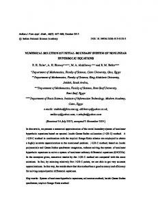
5 NUMERICAL EXAMPLE For a numerical example, we consider a non-convex boomerang-shaped boundary ? illustrated in Figure 1 and described by the parametric representation

x(t) = (cos t + 0:65 cos 2t ? 0:65 ; 1:5 sin t); 0  t  2:





Figure 1: Boomerang-shaped boundary for numerical example The boundary condition is given by

 

1 n?3 X F (x; t) = 81 t2 e?t = (n2 ? 9n + 8) 23n+3 Ln 2t n=0

The constants are a = 2 and b = 0:5 and the scaling parameter was chosen as  = 0:5.

x t

1.00

2.00

3.00

4.00

5.00

2N

n

= 15

Table 1: Numerical results = (?1 5 0) : ;

n

= 20

n

= 25

n

= 15

x

= (1:5; 2) n

= 20

n

= 25

16

0.030013

0.030590

0.030786

0.003506

0.003069

0.002453

32

0.030005

0.030583

0.030787

0.003509

0.003071

0.002454

16

0.058731

0.059014

0.058852

0.020987

0.020947

0.021506

32

0.058731

0.059014

0.058843

0.020987

0.020947

0.021508

16

0.054536

0.052994

0.052937

0.030385

0.031301

0.031316

32

0.054537

0.052991

0.052935

0.030384

0.031301

0.031316

16

0.036087

0.036305

0.036612

0.028977

0.028589

0.027707

32

0.036086

0.036306

0.036624

0.028977

0.028588

0.027704

16

0.020403

0.022546

0.022556

0.021816

0.020517

0.020772

32

0.020403

0.022551

0.022554

0.021816

0.020516

0.020772

14

REFERENCES

Table 1 gives some approximate values for the solution at the two points indicated by stars in Figure 1 obtained via the integral equation of the rst kind and shows that the method works satisfactorily. In particular, the numerical results exhibit the fast convergence with respect to the number 2N of quadrature points. In our future research we intend to establish a convergence and error analysis with respect to truncating the Laguerre{Fourier series after n terms. In addition, we need to investigate the stability with respect to the recursive computation of the Laguerre{ Fourier coecients. Finally, we wish to mention that the numerical results for the integral equation of the second kind for 2N = 32 agree with those for the integral equation of the rst kind.

REFERENCES [1] Arnold, D.N., and Noon, D.N.: Coercitivity of the single layer heat potential. J. Comput. Math. 7, 100-104 (1989). [2] Brebbia, C.A., Telles, J.C., and Wrobel, L.C.: Boundary Element Techniques. Springer-Verlag, Berlin Heidelberg New York 1984. [3] Chapko, R., and Kress, R.: On a quadrature method for a logarithmic integral equation of the rst kind. In: World Scienti c Series in Applicable Analysis { Vol. 2. Contributions in Numerical Mathematics (Agarwal, ed.) World Scienti c, Singapore, 127{140 (1993). [4] Chapko, R., and Kress, R.: Rothe's method for the heat equation and boundary integral equations. J. Integral Equations Appl. 9, 47{69 (1997). [5] Colton, D., and Kress, R.: Integral Equation Methods in Scattering Theory. Wiley-Interscience Publication, New York 1983. [6] Costabel, M.: Boundary integral operators for the heat equation. Integral Equations and Operator Theory 13, 498{552 (1990). [7] Galazyuk, V.: The method of Chebyshev{Laguerre polynomials in the initial boundary value problem for the nonlinear equation of second order. Dokl. Akad. Nauk. UkrSSR 1 (1981), 3{7 (in Russian). [8] Galazyuk, V., and Chapko, R.: The Chebyshev{Laguerre transformation and integral equation methods for the initial boundary value problems for the telegraph equation, Dokl. Akad. Nauk. UkrSSR 8 (1990), 11{14 (in Russian). [9] Hsiao, G.C., and Saranen, J.: Boundary integral solution of the two-dimensional heat equation. Math. Methods in Appl. Sciences 16, 87{114 (1993). [10] Kacur, J.: Method of Rothe in Evolution Equations. Teubnersche Verlagsanstalt, Leipzig 1985. [11] Kress, R.: Linear Integral Equations. Springer-Verlag, Berlin Heidelberg New York 1989. [12] Kress, R.: Inverse scattering form an open arc. Math. Meth. in the Appl. Sci. 17, (1994).

REFERENCES

15

[13] Kress, R., and Sloan, I.H.: On the numerical solution of a logarithmic integral equation of the rst kind for the Helmholtz equation. Numer. Math. 66, 199{214 (1993). [14] Lebedev, N.N.: Special Functions and Their Applications. Prentice-Hall, Englewood Clis 1965. [15] Lubich, C., and Schneider, R.: Time discretizations of parabolic boundary integral equations. Numer. Math. 63, 455{481 (1992). [16] Lyudkevich, I.V., and Muzychuk, A.E.: The numerical solution of initial boundary value problems for the wave equation. Lecture Notes, Lviv University, Lviv 1990 (in Russian). [17] Pogorzelski, W.: Integral Equations and Their Applications. Pergamon Press, Oxford 1966. [18] Protter, M.H., and Weinberger, H.F.: Maximum Principles in Dierential Equations. Prentice-Hall, Englewood Clis 1967. [19] Rektorys, K.: The Method of Discretization in Time. D. Reidel Publishing Company, Dordrecht 1982. [20] Tricomi, F.G.: Vorlesungen uber Orthogonalreihen. Springer-Verlag, Berlin Gottingen Heidelberg 1955.